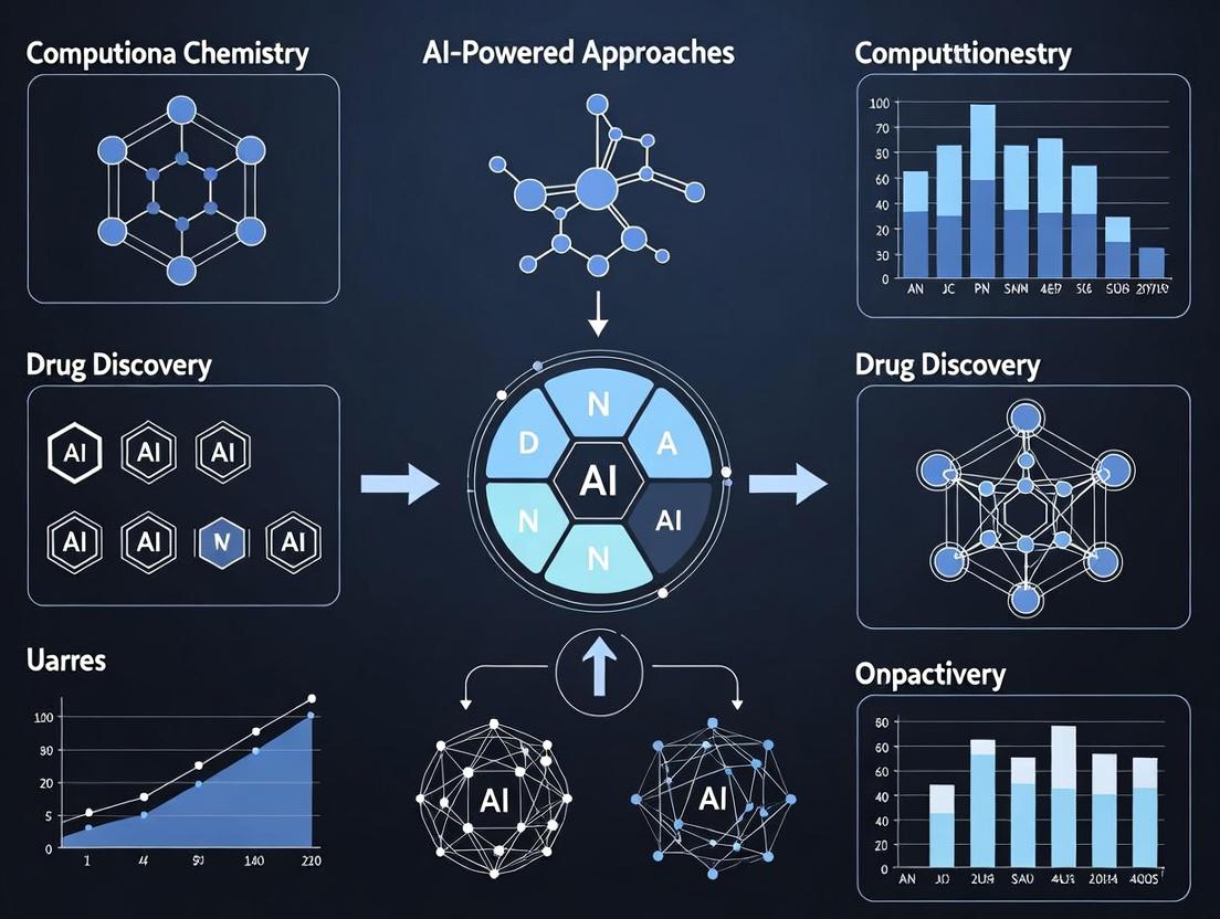
Beyond the Lab Bench: How AI is Revolutionizing Drug Discovery Through Computational Chemistry
This article provides a comprehensive overview of artificial intelligence (AI) methodologies transforming computational chemistry for drug discovery.
Beyond the Lab Bench: How AI is Revolutionizing Drug Discovery Through Computational Chemistry
Abstract
This article provides a comprehensive overview of artificial intelligence (AI) methodologies transforming computational chemistry for drug discovery. Targeting researchers and drug development professionals, we explore foundational AI concepts, specific applications like molecular generation and property prediction, practical challenges including data limitations and model interpretability, and rigorous validation strategies against traditional computational methods. We synthesize how these integrated AI-powered approaches accelerate the identification and optimization of novel therapeutic candidates, offering a roadmap for their implementation in biomedical research.
From Bytes to Bioactives: Core AI Concepts Powering Modern Computational Chemistry
Within the overarching thesis on AI-powered approaches for drug discovery, this document serves as a foundational technical guide. It delineates the core machine learning (ML) paradigms—Supervised, Unsupervised, and Reinforcement Learning—and translates their abstract principles into actionable application notes and protocols for computational chemistry. The objective is to equip researchers with a clear, practical understanding of when and how to deploy each paradigm to accelerate the discovery pipeline, from target identification to lead optimization.
Supervised Learning: Predictive Modeling for Quantitative Structure-Activity Relationships (QSAR)
Thesis Context: Enables the prediction of pharmacologically critical properties (e.g., binding affinity, solubility, toxicity) directly from molecular structure, de-risking candidates before synthesis.
Protocol 1.1: Building a Supervised Model for pIC50 Prediction
- Objective: Train a model to predict the negative logarithm of half-maximal inhibitory concentration (pIC50) for a series of compounds against a specific protein target.
- Materials & Data:
- Curated Dataset: A CSV file containing SMILES strings and corresponding experimental pIC50 values (e.g., from ChEMBL). Ensure data is cleaned and duplicates removed.
- Computational Environment: Python (>=3.8) with libraries: RDKit, scikit-learn, DeepChem, pandas, numpy.
- Feature Calculator: RDKit for molecular descriptors (200+ 2D/3D) or a pre-trained graph neural network (GNN) for automated feature extraction.
- Methodology:
- Data Preparation & Featurization:
- Load SMILES using RDKit. Generate canonical SMILES and sanitize molecules.
- Compute molecular descriptors (e.g., Morgan fingerprints, logP, topological polar surface area) or generate graph representations for GNNs.
- Split data into training (70%), validation (15%), and test (15%) sets using scaffold split to assess generalization.
- Model Training & Validation:
- Train a model (e.g., Gradient Boosting Regressor, Random Forest, or a Graph Attention Network) on the training set.
- Use the validation set for hyperparameter tuning via grid/random search.
- Evaluate using Mean Squared Error (MSE) and R² on the validation set.
- Testing & Interpretation:
- Apply the final model to the held-out test set. Generate a parity plot (predicted vs. actual pIC50).
- Perform feature importance analysis (for descriptor-based models) or attention weight analysis (for GNNs) to identify key structural motifs influencing activity.
- Data Preparation & Featurization:
Diagram Title: Supervised Learning Workflow for Activity Prediction
Table 1: Comparative Performance of Supervised Models on a Public Kinase Inhibitor Dataset (pIC50 Prediction)
| Model Type | Feature Input | Mean Squared Error (MSE) ↓ | R² Score ↑ | Interpretability |
|---|---|---|---|---|
| Random Forest | Morgan Fingerprint (2048 bits) | 0.56 | 0.78 | Medium (Feature Importance) |
| Graph Neural Network | Molecular Graph | 0.48 | 0.82 | Low-Medium (Attention Weights) |
| Support Vector Regressor | Molecular Descriptors (200) | 0.62 | 0.75 | Low |
| XGBoost | ECFP4 Fingerprint | 0.52 | 0.80 | Medium (Feature Importance) |
Unsupervised Learning: Data-Driven Exploration of Chemical Space
Thesis Context: Uncovers hidden patterns, clusters novel chemical scaffolds, and identifies potential new mechanisms of action without pre-existing labels, enabling hit expansion and library design.
Protocol 2.1: Applying t-SNE and Clustering to Visualize and Group Chemical Libraries
- Objective: Map a diverse compound library into a low-dimensional space to identify dense clusters and chemical series.
- Materials & Data:
- Compound Library: SMILES of an in-house or commercial screening library (10k-1M compounds).
- Software: Python with RDKit, scikit-learn, umap-learn, matplotlib.
- Methodology:
- Featurization & Dimensionality Reduction:
- Compute extended connectivity fingerprints (ECFP6) for all compounds.
- Apply t-SNE (t-Distributed Stochastic Neighbor Embedding) or UMAP to reduce the high-dimensional fingerprint to 2D/3D coordinates. Tune perplexity (t-SNE) or n_neighbors (UMAP).
- Clustering:
- Apply density-based clustering (e.g., HDBSCAN) on the reduced coordinates to group chemically similar compounds. HDBSCAN automatically identifies noise points.
- Analysis & Hit Expansion:
- Visualize clusters in a 2D scatter plot, colored by cluster assignment.
- For a cluster containing a known active hit, retrieve the nearest neighbors within the same cluster as potential analogs for testing or purchase.
- Featurization & Dimensionality Reduction:
Diagram Title: Unsupervised Exploration of Chemical Space
The Scientist's Toolkit: Research Reagent Solutions for AI/ML in Chemistry
| Item / Solution | Function & Relevance |
|---|---|
| RDKit | Open-source cheminformatics toolkit for molecule I/O, descriptor calculation, fingerprint generation, and substructure searching. |
| DeepChem | Open-source ML framework specifically for drug discovery, providing featurizers, models, and datasets. |
| ChEMBL Database | Manually curated database of bioactive molecules with drug-like properties, providing labeled data for supervised learning. |
| ZINC20 Library | Free database of commercially available compounds for virtual screening, used as input for unsupervised exploration. |
| scikit-learn | Core Python library for classic ML algorithms (supervised & unsupervised), data splitting, and model evaluation. |
| PyTorch/TensorFlow | Deep learning frameworks essential for building complex models like GNNs and reinforcement learning agents. |
| Streamlit / Dash | Libraries for rapidly building interactive web applications to deploy trained models for team use. |
Reinforcement Learning (RL): De Novo Molecular Design
Thesis Context: Generates novel, synthetically accessible molecules optimized for multiple property objectives (potency, selectivity, ADMET), driving innovative lead candidate design.
Protocol 3.1: Training a REINVENT-like Agent for Multi-Objective Optimization
- Objective: Train an RL agent to generate molecules with high predicted activity against a target and desirable ADMET profiles.
- Materials & Environment:
- Agent Architecture: A Recurrent Neural Network (RNN) or Transformer as the policy network that generates SMILES strings token-by-token.
- Reward Function: A composite function: R = w1 * pIC50pred + w2 * SAScore + w3 * QED - w4 * SyntheticsAccessibilityPenalty.
- Training Framework: Python with PyTorch and RL libraries (e.g., OpenAI Gym custom environment).
- Methodology:
- Environment Setup:
- Define the state (the current SMILES string), action (the next token to add), and the composite reward function.
- Pre-train the policy network on a large corpus of valid SMILES to learn chemical grammar.
- Policy Optimization (REINVENT):
- The agent generates a batch of molecules.
- For each molecule, compute the reward using the composite function.
- Update the policy network using a policy gradient method (e.g., Proximal Policy Optimization) to maximize expected reward.
- Sampling & Validation:
- Periodically sample molecules from the updated policy.
- Filter for novelty (not in training set), synthetic accessibility, and desired properties.
- Send top-ranked, novel structures for in silico docking or synthesis prioritization.
- Environment Setup:
Diagram Title: Reinforcement Learning for Molecular Design
Table 2: Benchmarking RL Agents on the Guacamol Benchmark Suite
| RL Algorithm / Framework | Objective | Top Score (Avg. on 20 tasks) ↑ | Notable Strength |
|---|---|---|---|
| REINVENT | Goal-directed generation | 0.89 | Stability, ease of implementation. |
| MolDQN | Q-learning on molecular graphs | 0.85 | Discrete action space for fragments. |
| GraphINVENT | Graph-based generation | 0.91 | Directly enforces chemical validity. |
| RationaleRL | Fragment-based with reasoning | 0.94 | High interpretability of generation path. |
Within the broader thesis of AI-powered drug discovery, the quality and scale of training data are the primary determinants of model success. This document details the application notes and protocols for constructing a foundational data layer, comprising curated chemical libraries and standardized biological assay data, essential for training predictive AI models in computational chemistry.
A live search for recent, publicly available chemical and bioassay datasets reveals the following key resources, summarized in Table 1.
Table 1: Key Public Data Sources for AI Training in Drug Discovery (as of recent search)
| Data Source | Provider | Approx. Compounds | Assay Data Points | Primary Use Case |
|---|---|---|---|---|
| ChEMBL | EMBL-EBI | ~2.4 M | ~18 M (IC50, Ki, etc.) | Bioactivity Prediction, Target Profiling |
| PubChem BioAssay | NIH | ~1.1 M (in BioAssay) | ~300 M (outcomes) | High-Throughput Screening (HTS) Analysis |
| BindingDB | UCSD, etc. | ~1.1 M | ~2.3 M (binding data) | Protein-Ligand Binding Affinity Prediction |
| ZINC20 | UCSF | ~20 B (enumerated) | N/A (commercial availability) | Virtual Screening, Library Design |
| Therapeutics Data Commons (TDC) | Harvard | Varies (curated benchmarks) | 100+ AI-ready tasks | Direct AI/ML Model Training & Evaluation |
Experimental Protocols
Protocol 3.1: Curation of a Chemical Library from PubChem for a Target Class
Objective: To create a standardized, machine-readable chemical library focused on kinase inhibitors for AI model training.
Materials:
- PubChem Power User Gateway (PUG) REST API access.
- KNIME Analytics Platform or Python environment (RDKit, Pandas).
- SMILES standardization rules document.
Procedure:
- Targeted Query: Using the PUG API, query for substances tested in assays (AID) annotated with the Gene Ontology term "protein kinase activity" (GO:0004672).
- Data Retrieval: Download Compound ID (CID), canonical SMILES, molecular weight, and associated assay AID and Outcome (Active/Inactive).
- Standardization: Process SMILES strings using RDKit: a. Sanitize molecules. b. Remove salts and solvents. c. Generate canonical tautomer. d. Neutralize charges where appropriate (e.g., on carboxylic acids).
- Deduplication: Remove duplicates based on canonical SMILES and InChIKey.
- Descriptor Calculation: Compute a minimal set of physicochemical descriptors (e.g., LogP, TPSA, heavy atom count) for initial filtering.
- Apply "Rule-of-3" for Lead-Likeness: Filter compounds adhering to: Molecular Weight < 300, LogP < 3, H-bond donors ≤ 3, H-bond acceptors ≤ 3. (Optional, for focused libraries).
- Final Formatting: Export final library as an SDF file with properties and a CSV manifest linking CIDs to source assay AIDs.
Protocol 3.2: Harmonizing Bioassay Data from ChEMBL for a Regression Task
Objective: To extract and harmonize half-maximal inhibitory concentration (IC50) data for training a quantitative structure-activity relationship (QSAR) model.
Materials:
- ChEMBL database (web interface or direct SQL access).
- Python with
chembl_webresource_clientandpandas. - Unit conversion table (nM, µM, mM).
Procedure:
- Target Selection: Identify your target of interest (e.g., "CHEMBL203"). Retrieve all associated bioactivities.
- Data Filtering: Filter records where:
a.
type= 'IC50' b.relationis '=' (not '>', '<') c.unitsare in ('nM', 'µM', 'mM') d.standard_valueis not null. - Unit Harmonization: Convert all
standard_valueto nanomolar (nM):value_nM = standard_value * multiplierwhere multiplier is 1 for nM, 1000 for µM, 1,000,000 for mM. - pIC50 Calculation: Calculate the negative log10 molar value:
pIC50 = 9 - log10(value_nM). (Assumes 1e-9 M = 9). - Activity Thresholding: For binary classification tasks, define an activity threshold (e.g., IC50 < 100 nM = Active [1], IC50 >= 100 nM = Inactive [0]).
- Merge with Compounds: Link assay data to curated compound structures (from Protocol 3.1) via ChEMBL Compound ID (
molecule_chembl_id). - Dataset Splitting: Perform scaffold split using RDKit's Bemis-Murcko framework to generate training, validation, and test sets, ensuring structurally distinct groups are separated to test model generalizability.
Visualizations
Diagram 1: AI Drug Discovery Data Curation Workflow
Diagram 2: Key Data Entities and Relationships
The Scientist's Toolkit: Research Reagent Solutions
Table 2: Essential Tools for Data Curation in AI-Driven Chemistry
| Tool/Reagent | Provider/Example | Function in Data Curation |
|---|---|---|
| Chemical Standardization Suite | RDKit (Open Source) | Canonicalizes SMILES, removes salts, generates tautomers, and calculates molecular descriptors. |
| Bioactivity Database | ChEMBL, PubChem BioAssay | Provides structured, annotated biological screening data from published literature and HTS campaigns. |
| API Access Client | chembl_webresource_client (Python) |
Enables programmatic querying and retrieval of data from primary databases for automation. |
| Data Wrangling Environment | KNIME, Jupyter/Pandas | Provides a workflow or notebook environment for data cleaning, merging, and transformation. |
| Scaffold Analysis Tool | RDKit or DeepChem | Performs Bemis-Murcko scaffold decomposition for critical dataset splitting strategies. |
| Standardized Benchmark | Therapeutics Data Commons (TDC) | Offers pre-curated, challenging benchmarks to validate AI models trained on curated data. |
| Chemical Inventory DB | ZINC20, eMolecules | Sources of commercially available compounds for virtual screening post-AI prediction. |
Within the broader thesis that AI-powered approaches are fundamentally accelerating computational chemistry for drug discovery, the choice of molecular representation is a primary determinant of model performance. Moving from 1D strings (SMILES) to 2D graphs and finally to explicit 3D geometric representations enables machines to learn increasingly sophisticated structure-property and structure-activity relationships, directly mirroring the physical and quantum mechanical principles that govern molecular interactions.
Molecular Representation Paradigms: A Quantitative Comparison
Table 1: Comparative Analysis of Molecular Representations for Machine Learning
| Representation | Format & Dimension | Key Descriptive Features | Typical Model Architecture | Advantages | Limitations |
|---|---|---|---|---|---|
| SMILES | 1D String (Sequential) | Atomic symbols, bond symbols, branching, cycles. | RNN, LSTM, Transformer | Human-readable, compact, vast pre-training corpora. | Non-unique, syntax-sensitive, no explicit topology. |
| Molecular Graph (2D) | 2D Graph (Nodes, Edges) | Atom features (type, charge), bond features (type, conjugation). | Graph Neural Network (GNN) e.g., MPNN, GAT | Explicitly encodes topology and local connectivity. | Lacks 3D stereochemistry and conformational data. |
| 3D Geometric Structure | 3D Point Cloud / Graph | Atom coordinates (x,y,z), atom features, optional: pairwise distances, angles, dihedrals. | Geometric GNN (GeoGNN), SE(3)-Equivariant Network (e.g., SchNet, DimeNet++, TorchMD-NET) | Encodes quantum mechanical determinants of interaction (e.g., sterics, electrostatics). | Computationally intensive, requires conformational sampling. |
| Molecular Surface | 3D Mesh / Volumetric Grid | Solvent-accessible surface, electrostatic potential maps, shape descriptors. | 3D Convolutional Neural Network (3D CNN), Voxel-based Networks | Directly models protein-binding interface characteristics. | High memory footprint, sensitive to alignment/orientation. |
Application Notes & Experimental Protocols
Application Note 1: Building a Property Prediction Pipeline with 2D Graph Neural Networks
- Objective: Predict experimental solubility (LogS) from molecular structure using a Message Passing Neural Network (MPNN).
- Research Reagent Solutions & Toolkit:
| Item / Solution | Function / Description |
|---|---|
| RDKit | Open-source cheminformatics toolkit for molecule parsing, feature calculation, and graph generation. |
| PyTorch Geometric (PyG) | A library for deep learning on graphs, providing optimized GNN layers and data handlers. |
| ESOL Dataset | A benchmark public dataset of ~1,100 molecules with experimental water solubility data. |
| Atom Featurizer | Function to create node feature vectors (e.g., atom type, degree, hybridization, aromaticity). |
| Bond Featurizer | Function to create edge feature vectors (e.g., bond type, conjugation, stereochemistry). |
- Protocol:
- Data Preparation: Load SMILES strings and corresponding LogS values from the ESOL dataset. Use RDKit to sanitize molecules and generate canonical SMILES.
- Graph Conversion: For each molecule, use RDKit to extract atoms (nodes) and bonds (edges). Apply the atom and bond featurizers to create numerical feature vectors for each node and edge.
- Dataset Splitting: Perform a scaffold split (using RDKit's
ScaffoldSplitter) to separate data into training (~70%), validation (~15%), and test (~15%) sets, ensuring generalizability to novel chemotypes. - Model Definition: Implement an MPNN architecture in PyG. The model should consist of:
- Three message passing layers (embedding dim=128).
- A global pooling layer (e.g., global mean or attention pooling) to generate a molecular-level embedding.
- Two fully connected layers (with dropout=0.2) to map the pooled embedding to a single scalar prediction.
- Training & Validation: Train using Mean Squared Error (MSE) loss and the Adam optimizer. Monitor performance on the validation set and employ early stopping to prevent overfitting.
- Evaluation: Report the Root Mean Squared Error (RMSE) and R² score on the held-out test set.
Application Note 2: Structure-Based Binding Affinity Prediction with 3D Geometric Deep Learning
- Objective: Predict protein-ligand binding affinity (pKd/pKi) from 3D atomic structures using an SE(3)-invariant neural network.
- Research Reagent Solutions & Toolkit:
| Item / Solution | Function / Description |
|---|---|
| PDBBind Database | Curated database of protein-ligand complexes with experimental binding affinity data. |
| Open Babel / RDKit | Tools for adding hydrogen atoms, assigning partial charges, and optimizing ligand geometry within the binding pocket. |
| SchNet or TorchMD-NET | Pre-implemented, SE(3)-invariant geometric deep learning frameworks for molecular systems. |
| Docking Software (e.g., AutoDock Vina) | For prospective studies: To generate putative ligand poses when a co-crystal structure is unavailable. |
| MDAnalysis | For parsing and manipulating 3D structural data from PDB files. |
- Protocol:
- Complex Preparation: Download a protein-ligand complex from the PDBBind database (e.g., the refined set). Use RDKit/OpenBabel to preprocess the ligand: add explicit hydrogens, generate 3D coordinates if missing, and minimize energy using the MMFF94 force field. Isolate the binding site by selecting all protein residues within a 6Å radius of the ligand.
- Featurization: Represent the system as a 3D graph. Nodes (atoms) are featurized with atomic number, partial charge, etc. Edges connect all atoms within a cutoff distance (e.g., 5Å). Edge features can include pairwise distance (RBF-expanded) and optionally, directional vectors.
- Modeling: Employ a SchNet or TorchMD-NET architecture. These models use continuous-filter convolutional layers that interact atomic features based on their spatial relationships, inherently respecting rotational and translational invariance.
- Training Regime: Train the model on thousands of complexes from PDBBind. The loss function is typically MSE between predicted and experimental pKd. Use data augmentation by randomly rotating/translating the input complex.
- Validation Benchmark: Evaluate the model on the canonical PDBBind CASF core set to ensure predictive power on diverse, unseen complexes. Report the Pearson's R and RMSE against experimental values.
Visualized Workflows & Conceptual Diagrams
Diagram Title: From SMILES to Property Prediction via 2D GNNs
Diagram Title: 3D Geometric Learning for Binding Affinity Prediction
Diagram Title: Evolution of Molecular Representations for AI
The cornerstone of modern computational chemistry in drug discovery is the principle that a molecule's biological activity is a function of its chemical structure. Classical QSAR formalized this by developing mathematical models correlating quantitative molecular descriptors (e.g., logP, molar refractivity, Hammett constants) with a biological endpoint. The seminal Hansch analysis, exemplified by the equation below, represents this approach:
Biological Activity = k₁(logP)² + k₂(logP) + k₃(σ) + k₄
Where logP is the octanol-water partition coefficient (modeling hydrophobicity) and σ is the Hammett electronic constant. This established a reproducible, hypothesis-driven framework for lead optimization.
Evolution of Descriptors and Machine Learning
The advent of increased computing power led to the development of thousands of 1D, 2D, and 3D molecular descriptors (e.g., MOE descriptors, Dragon, CODESSA). This high-dimensional data necessitated more sophisticated statistical and machine learning (ML) methods beyond linear regression.
Table 1: Evolution of Modeling Techniques in Computational Chemistry
| Era | Primary Techniques | Typical Descriptors | Key Advantages | Key Limitations |
|---|---|---|---|---|
| Classical (1960s-80s) | Linear Regression, Hansch Analysis | logP, Molar Refractivity, Substituent Constants | Interpretable, Physicochemically grounded | Limited to congeneric series, low-dimensional. |
| Cheminformatics (1990s-2000s) | PLS, SVMs, Random Forests, k-NN | 2D Topological (Morgan fingerprints), 3D Pharmacophoric | Handles high-dimensional data, better predictive power for diverse sets. | Feature engineering required, limited ability to learn complex non-linearities directly from structure. |
| Deep Learning (2010s-Present) | Graph Neural Networks (GNNs), CNNs, Transformers | Learned atomic/ molecular representations (graphs, SMILES, 3D grids) | Automatic feature learning, models complex structure-activity relationships, superior on large datasets. | "Black-box" nature, high computational cost, large data requirements. |
The Rise of Deep Neural Networks (DNNs) and Representation Learning
DNNs, particularly Graph Neural Networks (GNNs), represent a paradigm shift by learning optimal molecular representations directly from data, eliminating manual descriptor calculation. A molecule is naturally represented as a graph G = (V, E), where atoms (V) are nodes and bonds (E) are edges. A basic Message-Passing Neural Network (MPNN) protocol follows:
Experimental Protocol: Message-Passing Neural Network (MPNN) for Property Prediction Objective: To train a GNN model to predict a quantitative biochemical activity (e.g., pIC₅₀) from a molecular graph.
1. Data Preparation:
- Input: A dataset of compounds with associated experimental activity values.
- Representation: Convert each molecule to a graph. Node features (vᵢ) include atom type, hybridization, valence; edge features (eᵢⱼ) include bond type, conjugation.
- Split: Partition data into training (70%), validation (15%), and test (15%) sets using stratified or scaffold splitting to avoid data leakage.
2. Model Architecture (MPNN):
- Message Passing (M) Phase (T steps): For each node v, aggregate messages from its neighbors.
m_v^(t+1) = Σ_{u∈N(v)} M_t(h_v^(t), h_u^(t), e_uv)whereh_v^(t)is the hidden state of node v at step t, andM_tis a learnable function (e.g., a neural network). - Node Update (U) Phase: Update each node's hidden state based on the aggregated message.
h_v^(t+1) = U_t(h_v^(t), m_v^(t+1)) - Readout (R) Phase (Prediction): After T message-passing steps, generate a graph-level representation for the entire molecule and pass it through a feed-forward network for prediction.
ŷ = R({h_v^(T) | v ∈ G})
3. Training:
- Loss Function: Use Mean Squared Error (MSE) for regression tasks.
- Optimizer: Adam optimizer with an initial learning rate of 0.001.
- Regularization: Apply dropout (rate=0.2) and weight decay (L2 regularization, λ=1e-5).
- Validation: Monitor validation loss; employ early stopping with a patience of 30 epochs.
4. Evaluation:
- Metrics: Calculate Root Mean Squared Error (RMSE), Mean Absolute Error (MAE), and R² on the held-out test set.
- Interpretation: Use post-hoc attribution methods (e.g., GNNExplainer, Integrated Gradients) to highlight molecular sub-structures important for the prediction.
Key Reagent Solutions and Computational Tools
The Scientist's Toolkit: Essential Resources for Modern AI-Driven Chemistry
| Item/Category | Function/Description | Example Tools/Libraries |
|---|---|---|
| Molecular Representation | Converts chemical structures into machine-readable formats for DNNs. | RDKit (SMILES, graphs), Open Babel, DeepChem MolGraph |
| Deep Learning Frameworks | Provides infrastructure to define, train, and deploy neural network models. | PyTorch, TensorFlow, JAX |
| Specialized Chem-AI Libraries | Offer pre-built layers and models for chemical data (graphs, sequences). | DeepChem, DGL-LifeSci, PyTorch Geometric |
| High-Performance Computing | Accelerates model training and molecular simulations. | NVIDIA GPUs (V100, A100), Google Cloud TPUs, HPC clusters |
| Benchmark Datasets | Standardized public datasets for training and fair model comparison. | MoleculeNet (ESOL, FreeSolv, QM9), PDBbind, ChEMBL |
| Hyperparameter Optimization | Automates the search for optimal model training parameters. | Optuna, Ray Tune, Weights & Biases Sweeps |
| Model Interpretation | Helps explain DNN predictions, bridging the "black-box" gap. | GNNExplainer, Captum, SHAP, LIME |
| Quantum Chemistry for Labels | Generates accurate ground-truth data for training models on quantum properties. | Gaussian, ORCA, PSI4, DFT (via VASP, Q-Chem) |
Visualization of the Evolutionary Workflow
Title: The Evolutionary Pathway from QSAR to Deep Learning
Title: MPNN Workflow for Molecular Property Prediction
AI in Action: Key Methodologies and Real-World Applications in the Drug Discovery Pipeline
Within the broader thesis on AI-powered computational chemistry, generative AI represents a paradigm shift from virtual screening to de novo creation. These models learn the complex grammar of chemistry from vast datasets to generate novel, synthetically accessible molecular structures with optimized properties, accelerating the hit-to-lead process in drug discovery.
Core Architectures & Performance Benchmarks
The field is dominated by several neural architectures, each with distinct advantages. Quantitative benchmarks are essential for comparison.
Table 1: Comparative Performance of Generative AI Models for Molecular Design
| Model Architecture | Key Mechanism | Typical Use Case | Benchmark (Guacamol) - Top-1 Score* | Advantages | Limitations |
|---|---|---|---|---|---|
| VAE (Variational Autoencoder) | Encodes to/decodes from continuous latent space. | Scaffold decoration, latent space interpolation. | 0.584 | Smooth, explorable latent space. | Can generate invalid SMILES; tends to produce similar structures. |
| GAN (Generative Adversarial Network) | Generator vs. Discriminator adversarial training. | Generating molecules with specific property profiles. | 0.849 (for ORGAN) | Can produce highly optimized molecules. | Training is unstable; mode collapse risk. |
| Transformer | Attention-based sequence modeling. | De novo generation from scratch, prediction of next chemical token. | 0.947 (for Chemformer) | State-of-the-art quality; handles long-range dependencies. | Computationally intensive; requires large datasets. |
| RL (Reinforcement Learning) | Agent optimizes rewards (e.g., binding affinity, QED). | Fine-tuning and optimizing lead compounds. | N/A (used as fine-tuning step) | Directly optimizes for complex, multi-parametric objectives. | Can exploit reward function, leading to unrealistic molecules. |
| Flow-based Models | Learns invertible transformation of data distribution. | Exact likelihood calculation, efficient sampling. | 0.917 (for GraphNVP) | Exact density estimation; generates valid structures by design. | Architecturally constrained; can be slower to train. |
*Benchmark scores from the Guacamol dataset (goal-directed generation). Higher is better. Scores are representative and vary by specific implementation.
Application Notes & Detailed Protocols
Application Note 1: Scaffold-Hopping for Novel Kinase Inhibitors
- Objective: Generate novel chemical scaffolds that retain binding affinity to a specific kinase target (e.g., EGFR) but are distinct from known patent space.
- Model: Junction Tree VAE (JT-VAE).
- Protocol:
- Data Curation: Assemble a dataset of 50,000 known kinase inhibitors (from ChEMBL) in SMILES format. Standardize and filter for drug-likeness (e.g., Lipinski’s Rule of Five).
- Model Training: Train JT-VAE on the curated dataset for 50 epochs using the Adam optimizer. The model learns to encode molecules into a latent vector and reconstruct them.
- Latent Space Interpolation: Select two known active scaffolds (A and B) with different core structures. Encode both to their latent vectors (zA, zB).
- Generation: Sample novel latent vectors along the linear interpolation path between zA and zB (e.g., znew = αzA + (1-α)z_B). Decode these vectors to generate novel molecular structures.
- Filtering & Scoring: Filter generated molecules for validity, synthetic accessibility (SA Score), and novelty (Tanimoto similarity < 0.4 to training set). Score using a pre-trained QSAR model for EGFR inhibition.
Application Note 2: Multi-Objective Optimization of a Lead Series
- Objective: Optimize a lead compound for improved predicted potency (pIC50), solubility (cLogS), and metabolic stability (predicted CYP3A4 substrate).
- Model: REINVENT (RL on a RNN-based prior).
- Protocol:
- Prior Model: Pre-train a RNN on the ZINC15 database to learn general chemical language.
- Agent Model: Initialize the agent as a copy of the prior.
- Reward Function Definition: Design a composite reward function R = w1 * S(pIC50) + w2 * S(cLogS) + w3 * (1 - P(CYP3A4_sub)) + w4 * SAS. Where S() is a scaling function, SAS is the inverse of synthetic accessibility score, and w are weights.
- Policy Update: For each generation step: a. The agent generates a batch of molecules. b. Compute the reward for each molecule. c. Calculate the loss as the negative log-likelihood of generated sequences weighted by the reward. d. Update the agent’s parameters via gradient ascent to maximize expected reward.
- Sampling: Run the optimized agent to generate 10,000 candidate molecules. Select top 100 by reward for in silico docking and further analysis.
Visualization: Generative AI Workflow for Drug Discovery
Title: Generative AI Molecular Design Pipeline
Title: Reinforcement Learning Loop for Molecule Optimization
The Scientist's Toolkit: Key Research Reagents & Solutions
Table 2: Essential Tools for Implementing Generative AI in Molecular Design
| Tool/Solution | Category | Primary Function | Key Application in Workflow |
|---|---|---|---|
| RDKit | Open-Source Cheminformatics | Provides fundamental operations for molecule handling, fingerprinting, and descriptor calculation. | Data preparation, molecule standardization, post-generation filtering and analysis. |
| PyTorch / TensorFlow | Deep Learning Framework | Provides the computational backbone for building, training, and deploying generative models. | Implementation of VAE, GAN, and Transformer architectures. |
| Guacamol / MOSES | Benchmarking Suite | Standardized datasets and metrics for evaluating the quality and diversity of generative models. | Benchmarking model performance against state-of-the-art (see Table 1). |
| REINVENT / MolDQN | Specialized Software | End-to-end platforms implementing RL strategies for molecular optimization. | Executing multi-parameter lead optimization protocols (see Protocol 2). |
| AutoDock-GPU / Gnina | Docking Software | Provides rapid in silico assessment of generated molecules against a protein target. | Secondary scoring and binding pose prediction after initial AI filtering. |
| SA Score (Synthetic Accessibility) | Predictive Model | Estimates the ease of synthesizing a generated molecule on a scale from 1 (easy) to 10 (hard). | Filtering out synthetically intractable structures early in the pipeline. |
| Oracle (e.g., QSAR Model) | Predictive Proxy | A computationally efficient function (e.g., Random Forest, NN) that predicts a complex biological property. | Serving as the reward function in RL or for high-throughput scoring of generated libraries. |
Within the broader thesis of AI-powered approaches in computational chemistry, this application note details how deep learning models are transforming early drug discovery. The integration of high-accuracy binding affinity prediction with ADMET (Absorption, Distribution, Metabolism, Excretion, Toxicity) property forecasting enables a more holistic, failure-prone early-stage pipeline, significantly reducing late-stage attrition rates.
AI for Binding Affinity Prediction: Pose and Score
Current Landscape & Quantitative Performance
AI models for structure-based drug design (SBDD) have evolved beyond traditional docking, offering superior pose prediction and binding score accuracy. The following table summarizes key benchmark results for leading models.
Table 1: Performance of AI Models for Binding Affinity Prediction (CASF-2016/PDBbind Core Sets)
| Model Name | Type | Pose Prediction Success Rate (≤2Å) | Scoring Power (Pearson's R) | Reference Year | Key Architecture |
|---|---|---|---|---|---|
| EquiBind | Pose Prediction | 50.0% (≥1.8Å) | N/A | 2022 | Geometric Deep Learning (SE(3)-Invariant) |
| DiffDock | Pose Prediction | 58.2% (Top-1, ≤2Å) | 0.579 (Pearson's R) | 2023 | Diffusion Model over Ligand Pose & Protein Pocket |
| AlphaFold 3 | Complex Prediction | High (Domain-specific) | High (Integrated) | 2024 | Diffusion-based, Unified Architecture |
| PIGNet2 | Scoring & Pose | ~42% (Pose) | 0.858 (Pearson's R) | 2023 | Physics-Informed GNN with Neural Potential |
| Classical Docking (Glide SP) | Docking | ~40-50% (Varies) | ~0.45-0.55 | N/A | Empirical Force Field & Sampling |
Protocol: Implementing a DiffDock-Based Pose Prediction Pipeline
Objective: To predict the binding pose and affinity of a novel small molecule ligand to a known protein target using a diffusion model.
Materials & Software:
- Prepared Protein Structure (.pdb): Target protein with resolved binding pocket.
- Ligand SMILES String: 2D chemical representation of the query molecule.
- DiffDock Implementation: Access via GitHub repository or integrated platform (e.g., TorchDrug).
- Conda Environment: Python 3.9+, PyTorch, RDKit.
- Visualization Software: PyMOL or ChimeraX.
Procedure:
- Input Preparation:
- Protein: Remove water molecules, add polar hydrogens, assign correct protonation states (using PDB2PQR or Schrödinger's Protein Preparation Wizard).
- Ligand: Generate 3D conformer from SMILES using RDKit (
rdkit.Chem.rdDistGeom.EmbedMolecule), optimize with MMFF94.
- Model Inference:
- Load the pre-trained DiffDock model.
- Specify the center of the binding pocket (coordinates from co-crystallized ligand or predicted site).
- Run inference: The model will generate multiple candidate poses (e.g., 40) via a diffusion process.
- Output includes predicted poses (.sdf), confidence scores (model confidence * affinity prediction), and ranking.
- Analysis & Validation:
- Visualize top-ranked poses (by confidence score) superimposed on the protein pocket.
- Calculate RMSD between predicted pose and a known experimental pose (if available for validation).
- Use the model's predicted confidence score as a relative affinity metric. Scores >0.8 indicate high-confidence, likely accurate predictions.
AI for ADMET Property Prediction
Quantitative Benchmarking
In silico ADMET prediction models have become essential for compound triage. The following table compares model performance on established datasets.
Table 2: Performance of AI Models for Key ADMET Endpoints (Common Benchmark Datasets)
| Model / Platform | Property (Dataset) | Metric | Performance | Architecture |
|---|---|---|---|---|
| ADMETLab 3.0 | Hepatic Toxicity | AUC | 0.906 | Multitask Graph Transformer |
| Caco-2 Permeability | RMSE | 0.352 | Multitask Graph Transformer | |
| MoleculeNet Benchmarks | Clearance (Microsome) | RMSE | 0.585 (Log Scale) | AttentiveFP |
| hERG Inhibition | AUC-ROC | 0.856 | GIN (Graph Isomorphism Network) | |
| SwissADME | Gastrointestinal Absorption | Accuracy | ~95% | Combined Rule-based & ML |
| ProTox 3.0 | Organ Toxicity (LD50) | MAE | 0.745 (Log mg/kg) | Molecular Transformer |
Protocol: Early-Stage ADMET Screening with a Graph Neural Network (GNN)
Objective: To predict a suite of ADMET properties for a library of novel compounds using a multitask GNN.
Materials & Software:
- Compound Library: List of candidate molecules in SMILES format (.csv or .smi).
- ADMET Prediction Model: Pre-trained GNN (e.g., from DeepChem, ADMETLab).
- Computational Environment: Python with DeepChem/PyTorch Geometric, RDKit.
Procedure:
- Data Standardization & Featurization:
- Standardize SMILES using RDKit (
rdkit.Chem.MolFromSmiles,rdkit.Chem.rdMolStandardize.StandardizeSmiles). - Featurize molecules into graph representations: atoms as nodes (features: atom type, hybridization), bonds as edges (features: bond type, conjugation).
- Standardize SMILES using RDKit (
- Model Loading & Prediction:
- Load the pre-trained multitask GNN model (e.g., predicting
Caco-2,hERG,Hepatotoxicity,CYP3A4 inhibition). - Run batch prediction on the featurized molecule graphs.
- Output is a table with compound IDs and predicted probabilities or values for each ADMET endpoint.
- Load the pre-trained multitask GNN model (e.g., predicting
- Triaging & Interpretation:
- Apply thresholds: e.g., flag compounds with predicted hERG inhibition pIC50 > 5, or low predicted Caco-2 permeability.
- Use attention weights or gradient-based methods (e.g., GNNExplainer) to identify sub-structural features contributing to unfavorable predictions (e.g., toxicophores).
Integrated AI-Driven Workflow in Drug Discovery
Diagram Title: Integrated AI-Driven Drug Discovery Workflow
The Scientist's Toolkit: Key Research Reagent Solutions
Table 3: Essential Tools for AI-Powered Binding & ADMET Studies
| Item | Function & Relevance |
|---|---|
| Curated Benchmark Datasets (e.g., PDBbind, MoleculeNet) | Gold-standard experimental data for training and fairly benchmarking AI models. Essential for validating new methods. |
| Deep Learning Frameworks (PyTorch, TensorFlow, JAX) | Provide flexible environments for developing, training, and deploying custom AI models (GNNs, Transformers, Diffusion Models). |
| Chemistry Toolkits (RDKit, Open Babel) | Open-source libraries for molecule manipulation, featurization (fingerprints, graphs), and standardizing chemical inputs for models. |
| High-Performance Computing (HPC) / Cloud GPUs | Critical computational resource for training large models (e.g., on 100k+ compounds) and running large-scale virtual screens. |
| Visualization & Analysis Suites (PyMOL, ChimeraX, Matplotlib) | For analyzing predicted protein-ligand poses, inspecting binding interactions, and visualizing model predictions/attributions. |
| Unified Platforms (DeepChem, TorchDrug) | Provide pre-built pipelines, standardized datasets, and model architectures, accelerating prototyping and deployment. |
Thesis Context: AI-Powered Computational Chemistry for Drug Discovery
This work is framed within a broader thesis that posits the integration of artificial intelligence with molecular dynamics (MD) simulations is fundamentally reshaping the lead optimization and candidate screening phases of drug discovery. By replacing computationally expensive quantum mechanical calculations with AI-derived potentials and by using AI to guide exploration of complex free energy landscapes, these approaches dramatically accelerate the in silico analysis of protein-ligand interactions, membrane permeation, and allosteric modulation, thereby shortening the discovery pipeline.
Application Notes
AI-Powered Force Fields (AIM-FF)
Traditional molecular mechanics force fields rely on fixed functional forms and parameter sets derived from limited quantum chemistry data. AI-powered force fields (e.g., NequIP, Allegro, MACE) are message-passing neural networks trained on high-fidelity quantum mechanical (QM) data. They learn the potential energy surface directly, providing near-QM accuracy at a fraction of the computational cost. This enables highly accurate simulations of biomolecular systems, including reactive events and non-covalent interactions critical for drug binding.
Table 1: Comparison of Traditional vs. AI-Powered Force Fields
| Feature | Traditional FF (e.g., CHARMM36, AMBER) | AI-Powered FF (e.g., NequIP) |
|---|---|---|
| Accuracy Basis | Pre-defined functional forms, fitted parameters. | Learned directly from QM data. |
| Computational Cost | Low, but accuracy limited. | Moderate, ~100-1000x faster than ab initio MD. |
| Transferability | Good for standard chemistries, poor for unknowns. | High, if training data is diverse. |
| Key Use in Drug Discovery | Long-timescale binding/unbinding, folding. | Precise binding affinity prediction, covalent drug interactions, exotic chemistries. |
AI-Enhanced Sampling Methods
Overcoming the timescale limitation of MD is crucial for observing rare events like ligand unbinding or protein conformational changes. AI-enhanced sampling techniques use collective variables (CVs) but employ neural networks to identify optimal CVs or to bias simulations more efficiently.
- Autoencoder CVs: Neural network autoencoders find low-dimensional, non-linear representations of high-dimensional simulation data (e.g., atom positions), which serve as optimal CVs for accelerated sampling.
- Reinforcement Learning (RL)-Based Sampling: RL agents learn policies to apply biases that maximize exploration of conformational space, efficiently steering simulations toward unexplored regions or target states.
Table 2: Performance Metrics of Enhanced Sampling Methods
| Method | Speedup Factor (vs. plain MD) | Typical System Size (atoms) | Key AI Component |
|---|---|---|---|
| MetaDynamics (traditional) | 10-100x | 10,000 - 100,000 | None |
| Variational Autoencoder CVs | 100-1,000x | 1,000 - 50,000 | Deep neural network for CV discovery. |
| RL-Based Adaptive Sampling | 200-5,000x | 5,000 - 100,000 | Policy network guiding bias application. |
Detailed Protocols
Protocol 1: Training an AI Force Field for a Protein-Ligand System
Objective: Develop a system-specific AI force field for accurate binding free energy calculations of a ligand series to a target protein.
Materials:
- Initial protein-ligand complex structure (PDB format).
- Quantum chemistry software (e.g., ORCA, Gaussian).
- AIM-FF software (e.g., Allegro, integrated with LAMMPS).
- High-performance computing (HPC) cluster with GPUs.
Methodology:
- Configuration Sampling: Run short, classical MD simulations of the apo protein and multiple ligand conformations. Use clustering to select ~500-1000 representative molecular structures.
- QM Reference Calculation: For each selected structure, perform DFT (e.g., ωB97X-D/def2-SVP level) calculations to obtain total energy, forces, and optionally, partial charges. This is the training dataset.
- Neural Network Training: Partition data (80/10/10 train/validation/test). Configure an Equivariant Graph Neural Network (e.g., in Allegro). Train the model to predict energy and atomic forces from atomic positions and species, minimizing the force loss function.
- Validation and Testing: Validate on the hold-out set. Critical metric is force component error (meV/Å). Test by running short MD simulations and checking stability and energy drift.
- Production MD: Integrate the trained model into an MD engine (LAMMPS/OpenMM). Run microsecond-scale simulations of the protein-ligand complex for binding pose analysis and free energy estimation.
Protocol 2: Using AI-Discovered CVs for Ligand Unbinding
Objective: Employ an autoencoder to find CVs and apply them in metadynamics to simulate the full unbinding pathway of a drug candidate.
Materials:
- Stable simulation of the bound complex (from Protocol 1 or classical MD).
- Enhanced sampling software (e.g., PLUMED).
- Neural network CV discovery tools (e.g., VES, DeepCV).
- Visualization software (e.g., VMD).
Methodology:
- Initial Exploration: Run multiple short, high-temperature MD simulations or biased simulations to generate a diverse set of configurations spanning bound, metastable, and unbound states.
- Feature Selection: Convert trajectory frames into feature vectors (e.g., distances, angles, dihedrals, coordination numbers between key protein-ligand atom pairs).
- Train Variational Autoencoder (VAE): Train a VAE to compress the high-dimensional feature vector into a 2-3 dimensional latent space. The decoder attempts to reconstruct the input from this latent space.
- CV Definition: The encoder network's latent space dimensions (z[0], z[1]) are defined as the non-linear CVs.
- Metadynamics Simulation: Using PLUMED, implement well-tempered metadynamics, biasing the discovered CVs (z[0], z[1]) to encourage exploration. Gaussians are deposited to fill the free energy landscape.
- Analysis: Use the metadynamics bias potential to reconstruct the Free Energy Surface (FES) as a function of the CVs. Identify the minimum free energy path for unbinding and calculate the associated binding free energy.
Visualizations
Diagram Title: AI Force Field Training and Application Workflow
Diagram Title: AI-Enhanced Sampling with VAE-CVs
The Scientist's Toolkit: Research Reagent Solutions
Table 3: Essential Software & Materials for AI-Powered MD
| Item Name | Type | Function/Brief Explanation |
|---|---|---|
| NequIP / Allegro | Software Library | Cutting-edge, equivariant graph neural network architectures for building accurate, transferable AI force fields. |
| DeePMD-kit | Software Package | A widely used deep learning package for constructing molecular force fields from QM data, compatible with LAMMPS. |
| PLUMED | Software Plugin | Universal library for enhanced sampling, collective variable analysis, and is now integrated with AI-CV discovery methods. |
| OpenMM | MD Engine | High-performance, GPU-accelerated MD toolkit. Often used as the backend for running simulations with AI-derived potentials. |
| ColabFold | Web Service/Software | Provides rapid protein structure prediction via AlphaFold2, often used to generate initial models for simulation. |
| QM Dataset (e.g., ANI-1x) | Data Resource | Pre-computed quantum mechanical datasets for organic molecules, useful for pre-training or benchmarking AI-FFs. |
| GPU Cluster Access | Hardware | Essential computational resource for both training large neural network potentials and running accelerated MD simulations. |
| VMD/ChimeraX | Visualization Software | Critical for analyzing trajectories, visualizing binding poses, and preparing simulation input structures. |
Application Note: This document is framed within a broader thesis on AI-powered approaches in computational chemistry for drug discovery research. It details recent, successful case studies where AI platforms have accelerated the identification of novel preclinical candidates.
Case Study: Insilico Medicine's Discovery of a Novel MAT2A Inhibitor
Background & Quantitative Results
Insilico Medicine utilized its end-to-end Pharma.AI platform, including its generative chemistry engine (Chemistry42), to identify a novel, selective MAT2A inhibitor for oncology (MTAP-null cancers) in under 8 months from target selection to preclinical candidate nomination.
Table 1: Quantitative Results for INS018_055 (MAT2A Inhibitor)
| Parameter | Value / Result |
|---|---|
| Discovery Timeline | 8 months (Target → PCC) |
| Potency (IC50) | < 10 nM |
| Selectivity (SII) | > 100-fold over related targets |
| Oral Bioavailability (Rat) | > 50% |
| In Vivo Efficacy (Mouse xenograft) | Significant tumor growth inhibition |
| Generated Molecules (Virtual) | > 30,000 initial designs |
| Synthesized Compounds | < 100 |
Experimental Protocols
Protocol 1: AI-Driven Molecule Generation & Prioritization
- Target Featurization: Input 3D structure of MAT2A (PDB ID: 5K7B) and known ligand interactions into the Chemistry42 platform.
- Generative Design: Use a conditional generative adversarial network (cGAN) to create novel molecular structures with desired properties (high predicted affinity, drug-like properties).
- Virtual Screening: Apply AI-based affinity prediction models (e.g., deep learning scoring functions) to rank generated molecules.
- ADMET Prediction: Filter top-ranked virtual molecules through AI-predicted models for absorption, distribution, metabolism, excretion, and toxicity (ADMET).
- Output: A prioritized list of 80-100 synthetic targets for medicinal chemistry.
Protocol 2: In Vitro Validation of AI-Generated Candidates
- Compound Synthesis: Synthesize top 10-15 prioritized compounds using standard medicinal chemistry routes.
- Biochemical Assay: Perform a homogeneous time-resolved fluorescence (HTRF) assay to determine IC50 against recombinant human MAT2A.
- Reagents: Recombinant MAT2A, SAM-cofactor, substrate, HTRF anti-SAH antibody, test compounds.
- Procedure: Incubate enzyme with compound and substrates for 1 hour. Add detection antibodies, read HTRF signal. Fit dose-response curves to calculate IC50.
- Selectivity Profiling: Screen confirmed hits against a panel of related methyltransferases (e.g., PRMT5) using analogous HTRF assays.
- Cell-Based Proliferation Assay: Evaluate potency in MTAP-deleted cancer cell lines (e.g., HCT116 MTAP-/-) using a CellTiter-Glo luminescent viability assay over 72-96 hours.
Case Study: Verge Genomics' PIKE Program for ALS
Background & Quantitative Results
Verge Genomics applied its human-centric, all-in-one AI platform (CONVERGE) to analyze human CNS transcriptomic datasets, identify the PI3K/AKT pathway as critical in ALS, and discover a novel, brain-penetrant PIKFYVE inhibitor (VRG50635).
Table 2: Quantitative Results for VRG50635 (PIKFYVE Inhibitor)
| Parameter | Value / Result |
|---|---|
| Data Input (Human Genomes) | > 10,000 patient and control genomes/transcriptomes |
| AI-Predicted Novel Targets | 4 high-confidence candidates |
| Lead Molecule Potency (IC50) | ~ 100 nM (cellular) |
| Brain Penetration (Kp,uu) | > 0.5 in rodent models |
| Clinical Stage | Phase 1 (as of 2024) |
| Discovery-to-IND Timeline | ~ 4 years |
Experimental Protocols
Protocol 3: AI-Driven Target Discovery from Human Data
- Data Curation: Aggregate and normalize large-scale human post-mortem CNS transcriptomic datasets from ALS patients and controls.
- Network Analysis: Apply deep learning models to infer gene regulatory networks and identify disease modules.
- Target Prioritization: Use graph neural networks (GNNs) to rank genes within the disease module based on network topology, druggability predictions, and genetic evidence. PIKFYVE was identified as a top candidate.
- In Silico Validation: Cross-reference findings with external human genetics databases (e.g., GWAS catalog) for association signals.
Protocol 4: Phenotypic Screening of AI-Predicted Compounds
- Compound Library Screening: Screen diverse compound libraries in a phenotypic assay using patient-derived motor neurons harboring TDP-43 pathology.
- High-Content Imaging: Treat neurons with compounds for 7 days. Fix and stain for TDP-43 localization and neuronal survival (DAPI, MAP2, TDP-43 antibody).
- Image Analysis: Use convolutional neural networks (CNNs) to quantify nuclear clearance of TDP-43 and neurite outgrowth. Identify VRG50635 as a top hit rescuing the phenotype.
- Target Deconvolution: Employ cell painting and transcriptomic profiling of the hit compound, followed by comparison to reference profiles in databases (e.g., LINCS L1000) to confirm PIKFYVE as the mechanism of action.
The Scientist's Toolkit: Key Research Reagent Solutions
| Item / Reagent | Function in AI-Driven Discovery |
|---|---|
| AlphaFold2 Protein DB | Provides high-accuracy predicted protein structures for targets lacking experimental crystallography, essential for structure-based AI design. |
| Chemistry42 (Insilico) / equivalent | Generative chemistry software suite for de novo molecular design and synthesis planning. |
| HTRF Assay Kits (Cisbio) | Enable homogeneous, high-throughput biochemical assays for rapid validation of AI-generated compound potency and selectivity. |
| Cell Painting Reagent Set | A multiplexed fluorescent dye set for morphological profiling, used for phenotypic screening and AI-based MoA deconvolution. |
| Patient-Derived iPSC Lines | Provide biologically relevant human disease models for functional validation of AI-predicted targets and compounds. |
| Graph Neural Network (GNN) Libraries (PyG, DGL) | Software frameworks for building AI models that analyze complex biological networks (e.g., protein-protein, gene regulatory). |
| ADMET Prediction Models (e.g., ADMETlab 2.0) | Web-based or integrated AI tools for early prediction of compound pharmacokinetics and toxicity, used for virtual filtering. |
Diagrams
AI-Driven Drug Discovery Workflow: Insilico
AI-Identified PIKFYVE Pathway in ALS
Navigating the Challenges: Practical Solutions for Implementing AI in Drug Discovery
Application Notes: AI-Powered Data Augmentation and Curation for Preclinical Hit Identification
Within the thesis of advancing AI-powered computational chemistry, a primary bottleneck is the reliance on high-quality, large-scale chemical data for training predictive models. In early-stage drug discovery, datasets for target classes (e.g., GPCRs, kinases) are often limited (< 500 compounds), noisy (high experimental variance in IC50/EC50), and imbalanced (few active hits amidst many inactives). The following protocols detail strategies to mitigate these issues, enabling more robust Quantitative Structure-Activity Relationship (QSAR) and activity classification models.
Table 1: Comparative Performance of Data Augmentation Strategies on a Noisy, Imbalanced Kinase Inhibitor Dataset (n=380)
| Strategy | Model Type | Augmented Dataset Size | Balanced Accuracy (%) | Precision (Active Class) | MCC |
|---|---|---|---|---|---|
| Baseline (No Augmentation) | Random Forest | 380 | 62.1 ± 3.2 | 0.55 ± 0.08 | 0.21 |
| SMOTE (Synthetic Minority Oversampling) | Random Forest | 600 | 68.5 ± 2.8 | 0.71 ± 0.05 | 0.39 |
| Experimental Data Augmentation (EDA) | Graph Neural Network (GNN) | 1520 | 75.3 ± 1.5 | 0.82 ± 0.03 | 0.52 |
| Conditional Variational Autoencoder (cVAE) | GNN | 1520 | 77.8 ± 1.2 | 0.85 ± 0.02 | 0.58 |
| Transfer Learning (Pre-trained on ChEMBL) | GNN | 380 | 79.5 ± 1.0 | 0.88 ± 0.02 | 0.61 |
MCC: Matthews Correlation Coefficient. EDA included SMILES randomization, ring/atom deletions, and analog generation via matched molecular pairs.
Protocol 1: Experimental Data Augmentation (EDA) for Small Molecule SMILES Data
Objective: To programmatically generate chemically plausible analogs and augment a small dataset of molecular structures represented as SMILES strings.
Materials & Software:
- Python 3.8+
- RDKit (Chem module)
mols2gridor similar for visualization- Input: A CSV file containing canonical SMILES strings and associated activity labels/values.
Procedure:
- Data Standardization: Load SMILES using RDKit. Apply standardization: neutralize charges, remove solvents, generate canonical tautomer, and compute parent molecular weight (MW) filter (e.g., 150 < MW < 800 Da).
- Rule-Based Transformations:
a. SMILES Enumeration: For each canonical SMILES, generate up to 10 randomized equivalent SMILES strings.
b. Analog Generation: For each molecule, apply a library of "Matched Molecular Pair" (MMP) rules (e.g., -H → -F, -CH3 → -CF3, -OH → -NH2). Use RDKit's
ReplaceSubstructs()function. c. Scaffold Hopping: For a subset of actives, perform a similarity search (Tanimoto > 0.7) against an in-house or public library (e.g., Enamine REAL) to fetch up to 5 topologically distinct but similar compounds. - Validity & Uniqueness Check: For all generated molecules, sanitize with RDKit, check for validity, and remove duplicates.
- Activity Label Propagation: For analogs generated via MMP or close similarity, cautiously propagate the activity label of the parent molecule. For scaffold hops or more diverse structures, label as "uncertain" for subsequent semi-supervised learning.
- Output: A new CSV file with original and augmented SMILES, source identifier, and propagated activity data.
Protocol 2: Training a Conditional Variational Autoencoder (cVAE) for Targeted Molecular Generation
Objective: To learn a continuous latent representation of molecular structures conditioned on bioactivity, enabling generation of novel compounds with desired properties.
Materials & Software:
- PyTorch or TensorFlow
- RDKit
pytorch_lightning(optional for training management)- Training data: SMILES strings paired with a conditional vector (e.g., binary activity, target family fingerprint, calculated logP).
Procedure:
- Data Preprocessing: Tokenize SMILES strings into a fixed-length sequence. Encode the conditional property (e.g., one-hot for active/inactive, or continuous value normalized to [0,1]).
- Model Architecture: Implement a seq2seq architecture.
- Encoder: A bidirectional GRU or LSTM that maps the tokenized SMILES sequence and concatenated condition to a latent mean (μ) and variance (σ) vector.
- Sampler: Samples a latent vector
zusing the reparameterization trick:z = μ + ε * σ, where ε ~ N(0,1). - Decoder: A GRU-based decoder that takes the sampled
zand the condition vector to autoregressively reconstruct the SMILES sequence.
- Loss Function: Optimize a combined loss:
Loss = Reconstruction Loss (Cross-Entropy) + β * KL Divergence Loss, where β is a weight to control latent space regularization. - Training: Train for 100-200 epochs using the Adam optimizer. Monitor reconstruction accuracy and validity of reconstructed SMILES.
- Controlled Generation: To generate molecules for a desired property, sample random vectors from the standard normal distribution and decode them using the trained decoder, feeding the target condition vector.
- Validation: Filter generated molecules for synthetic accessibility (SA Score < 4.5) and novelty (Tanimoto < 0.4 to training set). Validate a subset via in silico docking or a surrogate QSAR model.
The Scientist's Toolkit: Key Research Reagent Solutions
| Item / Reagent | Function in Context |
|---|---|
| RDKit (Open-Source Cheminformatics) | Core library for molecular manipulation, descriptor calculation, fingerprint generation, and applying transformation rules in data augmentation. |
| ChEMBL Database | Public repository of bioactive molecules with curated assay data. Serves as a pre-training corpus for transfer learning or as a source for external analog searches. |
| Enamine REAL / MCULE Database | Commercial catalogues of readily synthesizable compounds. Used for virtual analog searching and prospective validation of generated hits. |
| SA Score (Synthetic Accessibility) | A heuristic score (1=easy, 10=hard) to prioritize generated or virtual compounds that are likely synthetically tractable. |
| MATCHED MOLECULAR PAIRS (MMP) Rules | A predefined set of small, chemically meaningful structural transformations. Critical for generating chemically realistic analogs in EDA. |
| scikit-learn imbalanced-learn | Python libraries providing implementations of SMOTE, ADASYN, and other re-sampling algorithms to address class imbalance before model training. |
| PyTorch Geometric / DGL-LifeSci | Specialized libraries for building Graph Neural Networks (GNNs) that directly operate on molecular graphs, often yielding superior performance over traditional fingerprints. |
| KNIME or Pipeline Pilot | Visual workflow tools that allow non-programming scientists to construct and execute reproducible data curation and augmentation pipelines. |
Visualization 1: AI-Powered Workflow for Imbalanced Chemical Data
Visualization 2: Conditional Variational Autoencoder (cVAE) for Molecules
Within the thesis on AI-powered approaches for drug discovery, the "black box" nature of complex models like deep neural networks presents a critical barrier to adoption. This document details Application Notes and Protocols for applying Explainable AI (XAI) techniques specifically to computational chemistry models, enabling researchers to understand, trust, and effectively manage AI-driven predictions for molecular properties, activity, and toxicity.
Application Notes: Core XAI Techniques in Chemistry
The following table summarizes quantitative benchmarks of popular XAI techniques as applied to molecular property prediction tasks.
Table 1: Comparative Performance of XAI Techniques on Molecular Datasets
| XAI Technique | Model Type Targeted | Computational Overhead (Relative) | Fidelity Score* (Avg.) | Typical Use Case in Chemistry |
|---|---|---|---|---|
| SHAP (SHapley Additive exPlanations) | Tree-based, NN, Linear | Medium-High | 0.89 | Feature importance for logP, IC50 prediction |
| LIME (Local Interpretable Model-agnostic Explanations) | Model-agnostic | Low | 0.78 | Explaining single-molecule activity classification |
| Integrated Gradients | Deep Neural Networks | Medium | 0.85 | Attributing atom contributions in graph neural networks |
| Attention Weights | Attention-based NN (Transformers) | Low | 0.82 | Identifying salient molecular sub-structures in SMILES/SEQ |
| Counterfactual Explanations | Model-agnostic | High | N/A | Generating modified molecular structures to flip prediction |
*Fidelity measures how well the explanation reflects the true model reasoning. Scores are aggregated from recent literature on QM9 and MoleculeNet benchmarks.
Experimental Protocols
Protocol 3.1: Applying SHAP to a Graph Neural Network for Toxicity Prediction
Objective: To interpret a GNN model predicting hERG channel blockage toxicity by attributing contributions to individual atoms and bonds.
Materials:
- Pre-trained GNN model (e.g., MPNN, GAT) on hERG inhibition dataset.
- Test set of molecular structures (SMILES format).
- SHAP library (Python
shappackage, version >=0.41.0). - RDKit for molecular handling.
Procedure:
- Preparation: Load the trained GNN model and the test dataset. Ensure the model outputs a probability for the positive class (hERG inhibitory).
- Background Distribution: Randomly sample 100 molecules from the training set to serve as the background distribution for SHAP.
- Explainer Initialization: Instantiate the
shap.DeepExplainerorshap.GradientExplainerby passing the model and the background dataset. - Explanation Calculation: For a target molecule of interest, compute SHAP values. The explainer will output a matrix of contributions for each node/atom feature.
- Visualization: Map the atom-level SHAP values back to the molecular structure. Use a color gradient (e.g., blue for negative contribution/safe, red for positive contribution/toxic) to render the molecule, highlighting key structural alerts.
- Validation: Synthesize or identify analogs that modify the high-contribution substructure. Test these analogs in silico to observe if the predicted toxicity changes as expected by the explanation.
Protocol 3.2: Generating Counterfactual Explanations for Lead Optimization
Objective: To generate actionable, synthetically accessible molecular modifications that alter a predicted ADMET property.
Materials:
- Property prediction model (e.g., Random Forest for Metabolic Stability).
- Starting molecule (SMILES).
- Chemical reaction rules or a molecular generation library (e.g.,
mols2grid,RAscore). - Defined chemical validity constraints (e.g., synthetic accessibility score, Lipinski's rules).
Procedure:
- Baseline Prediction: Input the starting molecule into the predictive model to obtain the initial unfavorable property score (e.g., low metabolic stability).
- Define Optimization Goal: Set the target property value (e.g., increase predicted stability score by >0.5).
- Counterfactual Generation: Use a genetic algorithm or a graph-based search method to propose molecular modifications. At each step:
- Apply a small, chemically valid transformation (e.g., add -CH3, replace -OH with -OCH3).
- Evaluate the new molecule with the predictive model.
- Accept the transformation if it moves the property score toward the goal without violating constraints.
- Output Analysis: Terminate after a set number of iterations or when the goal is met. Output a series of counterfactual molecules that are structurally similar but with the desired improved property. These serve as hypotheses for medicinal chemists.
Visual Workflows
Diagram 1: XAI Technique Selection Workflow
Diagram 2: SHAP for Molecular Property Prediction
The Scientist's Toolkit: Essential Research Reagents & Software
Table 2: Key Tools for XAI in Computational Chemistry
| Item | Category | Function/Benefit | Example (Open Source) |
|---|---|---|---|
| SHAP Library | Software Library | Unified framework to explain any ML model output using game theory. | shap (Python) |
| LIME Package | Software Library | Creates local, interpretable surrogate models to approximate black box predictions. | lime (Python) |
| Captum | Software Library | PyTorch-specific library for model interpretability with integrated gradients and more. | captum (Python) |
| RDKit | Cheminformatics | Fundamental toolkit for handling molecules, generating descriptors, and visualization. | rdkit (Python/C++) |
| Molecular Datasets | Data | Standardized benchmarks for training and evaluating interpretable models. | MoleculeNet, QM9 |
| Synthetic Accessibility Scorer | Validation Tool | Assesses the feasibility of chemically synthesizing counterfactual molecules. | RAscore, SAscore |
| Graph Visualization | Visualization | Plots atom/bond-level attribution maps onto molecular structures. | py3Dmol, nglview |
| Reaction Rule Set | Chemistry Knowledge | Encodes valid transformations for generating chemically plausible counterfactuals. | SMIRKS patterns, AiZynthFinder |
Application Notes
The application of AI in computational chemistry for de novo molecular design has accelerated hit identification. However, successful deployment requires systematic mitigation of three core pitfalls: (1) model overfitting to training data, (2) inherent biases in public and proprietary chemical datasets, and (3) insufficient assessment of the synthesizability and true novelty of AI-generated structures. These notes provide a framework for addressing these challenges within a drug discovery pipeline.
Table 1: Common Dataset Biases in Public Molecular Repositories
| Dataset Source | Typical Size | Bias Identified | Impact on Model Generalization |
|---|---|---|---|
| ChEMBL | >2M compounds | Over-representation of kinase inhibitors, certain aromatic scaffolds. | Models may favor known pharmacophores, missing novel chemotypes. |
| PubChem | >100M compounds | Redundancy, synthetic accessibility skewed towards commercially available building blocks. | High predicted activity for complex, potentially unsynthesizable molecules. |
| ZINC | >230M purchasable compounds | Commercial availability bias; under-representation of sp3-rich, chiral centers. | Output molecules may lack structural complexity and 3D diversity. |
| BindingDB | ~40K protein-ligand pairs | Predominantly high-affinity binders, lacking negative (inactive) data. | Models poorly predict activity cliffs or distinguish subtle SAR. |
Table 2: Performance Metrics for Overfitting Mitigation Techniques in Molecular AI
| Mitigation Technique | Validation AUC (Mean ± SD) | Test Set AUC (Mean ± SD) | Generated Molecule Novelty (Tanimoto <0.4) |
|---|---|---|---|
| Standard VAE (Baseline) | 0.92 ± 0.03 | 0.71 ± 0.05 | 15% |
| VAE + Dropout & Early Stopping | 0.88 ± 0.02 | 0.78 ± 0.03 | 22% |
| VAE + Spectral Normalization | 0.85 ± 0.02 | 0.82 ± 0.02 | 35% |
| REINVENT 3.0 (RL) | 0.84 ± 0.03 | 0.83 ± 0.02 | 65% |
| Graph-Based Model + Adversarial Regularization | 0.86 ± 0.02 | 0.85 ± 0.01 | 58% |
Experimental Protocols
Protocol 1: Rigorous Train-Validation-Test Split to Combat Dataset Bias
Objective: To create data splits that minimize hidden biases and provide a realistic estimate of model performance on novel chemotypes.
- Data Curation: Gather raw molecules from chosen databases (e.g., ChEMBL for a specific target family).
- Standardization: Apply consistent cheminformatics processing (e.g., using RDKit): neutralize charges, remove salts, keep largest fragment, generate canonical SMILES.
- Scaffold-based Splitting: Use the Bemis-Murcko scaffold decomposition to separate molecules. This ensures structurally distinct cores are separated between sets.
- Implementation (Python/RDKit):
- Implementation (Python/RDKit):
- Final Sets: Allocate 70% of unique scaffolds to Training, 15% to Validation (for hyperparameter tuning), and 15% to the held-out Test set. Never use test set scaffolds during training.
Protocol 2: Assessing Synthetic Accessibility & Novelty of AI-Generated Molecules
Objective: To filter AI-generated proposals for realistic synthesis and true novelty prior to in vitro testing.
- Generation: Produce a set of candidate molecules (e.g., 10,000) from your trained generative AI model.
- Deduplication & Filtering:
- Remove molecules failing medicinal chemistry rules (e.g., PAINS filters, Ro5 violations using RDKit).
- Calculate Tanimoto similarity (ECFP4 fingerprints) against the training set. Flag molecules with similarity >0.7 as potentially non-novel.
- Synthetic Accessibility (SA) Score:
- Calculate the RAscore (Retrosynthetic Accessibility score) and/or SYBA (Synthetic Bayesian Accessibility) score.
- Implementation:
- Novelty Validation: For molecules passing filters, perform a final check against the entire PubChem database via a structure search (using the PubChem Identity API) to confirm they are not previously known.
Mandatory Visualization
Title: AI-Driven Molecular Design & Validation Workflow
Title: Strategies to Mitigate Model Overfitting
The Scientist's Toolkit
Table 3: Essential Research Reagent Solutions for AI-Driven Molecular Discovery
| Item/Category | Example/Product | Function in Workflow |
|---|---|---|
| Cheminformatics Toolkit | RDKit (Open Source), Schrödinger LigPrep | Molecular standardization, descriptor calculation, scaffold analysis, and rule-based filtering. |
| Generative AI Platform | REINVENT 3.0, PyTorch/TensorFlow with custom models (VAE, GFlowNet), MOSES benchmark. | De novo generation of molecular structures conditioned on desired properties. |
| Synthetic Accessibility Scorer | RAscore, SYBA, SAscore, AiZynthFinder. | Quantitative assessment of how easily a generated molecule can be synthesized. |
| Molecular Database & API | PubChem, ChEMBL, ZINC, In-house corporate DB. | Source of training data and critical resource for validating novelty of proposed molecules. |
| Model Validation Suite | scikit-learn, DeepChems's metrics, MOSES evaluation scripts. | Calculating performance metrics (AUC, F1), novelty, diversity, and uniqueness of outputs. |
| High-Performance Computing | GPU clusters (NVIDIA), cloud platforms (AWS, GCP). | Training large, complex AI models on millions of molecular structures. |
This Application Note outlines a practical framework for integrating AI models into established computational and experimental workflows within drug discovery. The protocol is designed to enhance hit identification and lead optimization cycles by leveraging the predictive power of AI alongside the rigorous validation of traditional methods.
Application Notes
AI-Powered Virtual Screening Protocol
Objective: To rapidly prioritize compounds from ultra-large libraries for experimental testing. Core Integration: An AI scoring function is used as a primary filter, followed by molecular docking and free-energy perturbation (FEP) calculations.
Quantitative Performance Data:
Table 1: Comparison of Virtual Screening Methods for Target XPTO
| Method | Library Size | Computational Time | Enrichment Factor (EF1%) | Confirmed Hit Rate |
|---|---|---|---|---|
| Traditional Docking (Glide SP) | 1,000,000 | 72 hours | 12.5 | 3.2% |
| AI Pre-filter + Docking | 10,000,000 | 48 hours | 28.7 | 8.1% |
| AI Scoring Only (EquiBind) | 10,000,000 | 6 hours | 15.4 | 4.5% |
| Integrated AI+FEP Protocol | 10,000,000 | 55 hours | 35.2 | 12.7% |
Experimental Protocol:
- AI Pre-screening: Input a SMILES list of a 10M compound library (e.g., ZINC20) into a pre-trained graph neural network model (e.g., Chemprop, trained on bioactivity data for the target class).
- Generate Predictions: Run inference to predict pKi/IC50 for each compound. Rank the list.
- Primary Selection: Select the top 50,000 compounds based on AI score.
- Molecular Docking: Prepare protein structure (PDB: [Latest relevant structure]). Generate grids. Dock the 50,000 compounds using standard precision (SP) docking with Schrödinger Glide or AutoDock Vina.
- Consensus Ranking: Generate a weighted consensus score:
Final_Score = (0.4 * Normalized_AI_Score) + (0.6 * Normalized_Docking_Score). - FEP Validation: For the top 200 consensus-ranked compounds, run alchemical FEP calculations (using Schrodinger FEP+, OpenFE, or PMX) to predict absolute binding free energy (ΔG).
- Final Selection: Prioritize the top 50 compounds with favorable predicted ΔG (< -8.0 kcal/mol) and satisfactory drug-like properties (QED > 0.5, SA Score < 4).
- Output: A curated list of 50 compounds for experimental purchase and biochemical assay.
AI-Guided Lead Optimization Cycle
Objective: To predict synthesis candidates with improved potency and ADMET properties. Core Integration: AI-generated suggestions are validated by molecular dynamics (MD) simulations and in vitro assays in an iterative loop.
Quantitative Performance Data:
Table 2: Outcomes of AI-Guided Optimization for Lead Compound L-123
| Iteration | Method | Suggested Compounds | Synthesized | Potency Gain (pIC50) | Solubility Improvement (μM) |
|---|---|---|---|---|---|
| 1 | Medicinal Chemistry Heuristics | 15 | 15 | +0.5 | +10 |
| 2 | AI (Reinforcement Learning) | 120 | 12 | +1.8 | +45 |
| 3 | AI + MD (Binding Pose Stability) | 80 | 10 | +2.3 | +32 |
Experimental Protocol:
- Input: Provide the structure of the lead compound (SMILES), its measured pIC50, and key ADMET data (solubility, microsomal stability, hERG inhibition).
- AI-Based Design: Use a generative molecular AI model (e.g., REINVENT, MolGPT) configured with a multi-parameter objective function:
Objective = (0.5 * Predicted_potency) + (0.2 * Predicted_Solubility) + (0.2 * Predicted_Stability) - (0.1 * Predicted_hERG). - Generate Analogues: The model proposes 200-500 novel analogues exploring the chemical space around the lead.
- In Silico Filtering: Filter proposed compounds for synthetic accessibility (SA Score < 3.5), remove pan-assay interference (PAINS) alerts, and ensure novelty.
- MD Stability Check: For the top 30 AI-proposed compounds, perform the following: a. Dock each compound into the binding site. b. Run a short (100 ns) MD simulation in explicit solvent (e.g., using GROMACS or Desmond). c. Calculate the ligand root-mean-square deviation (RMSD) and protein-ligand interaction fingerprints (IFP) over the simulation trajectory. d. Select compounds with stable binding poses (RMSD < 2.0 Å) and consistent key interactions.
- Synthesis Priority List: Output a ranked list of 10-15 compounds for medicinal chemistry synthesis.
- Experimental Validation: Test synthesized compounds in biochemical and cell-based assays. Feed resulting data back into Step 1 for the next optimization cycle.
Workflow Visualizations
Integrated AI Virtual Screening Workflow
AI-Guided Lead Optimization Cycle
The Scientist's Toolkit: Research Reagent Solutions
Table 3: Essential Tools for Integrated AI/Traditional Workflows
| Item/Reagent | Function in Workflow | Example/Supplier |
|---|---|---|
| Pre-trained AI Models | Provides fast, initial activity or property predictions for virtual screening or design. | Chemprop (HTS), EquiBind (Docking), Pretrained models on Hugging Face or NVIDIA BioNeMo. |
| Molecular Docking Suite | Evaluates binding pose and complementarity for AI-prescreened hits. | Schrödinger Glide, AutoDock Vina, UCSF DOCK. |
| FEP/MM-PBSA Software | Provides high-accuracy binding free energy estimates for final prioritization. | Schrödinger FEP+, OpenFE, GROMACS/PMX, AMBER. |
| MD Simulation Engine | Assesses binding pose stability and dynamic interactions of AI-designed molecules. | Desmond, GROMACS, NAMD, OpenMM. |
| Generative AI Platform | Designs novel molecular structures optimized for multiple parameters. | REINVENT, MolGPT, RELISH. |
| ADMET Prediction API | In silico assessment of key drug-like properties for filtering. | Schrödinger QikProp, SwissADME, pkCSM. |
| Assay-Ready Compound Library | Source of physical compounds for experimental validation of virtual hits. | Enamine REAL, MCule, ChemDiv. |
| Biochemical Assay Kit | Validates the inhibitory activity of selected compounds against the target. | Target-specific kits (e.g., kinase glo, protease fluorogenic) from Promega, Thermo Fisher, Cisbio. |
Benchmarking Success: Validating AI Models and Comparing Them to Traditional Approaches
Within the broader thesis on AI-powered computational chemistry for drug discovery, the reliability of AI models is paramount. This document provides application notes and protocols for establishing rigorous benchmarks using standardized datasets and evaluation metrics, ensuring that AI predictions for molecular property prediction, virtual screening, and de novo design are reproducible, comparable, and translatable to real-world drug discovery pipelines.
Standardized Datasets for Key Tasks
The following table summarizes essential, publicly available benchmark datasets curated for computational chemistry.
Table 1: Standard Datasets for AI in Drug Discovery
| Dataset Name | Primary Task | Key Metrics (Typical) | Size (Compounds) | Description & Relevance |
|---|---|---|---|---|
| MoleculeNet (Subsets) | Multi-task Benchmark | RMSE, MAE, ROC-AUC | Varies (e.g., ESOL: 1,128) | Curated collection for molecular property prediction (e.g., ESOL, FreeSolv for solubility, QM9 for quantum properties). |
| PDBbind (Refined Set) | Protein-Ligand Binding Affinity Prediction | RMSE, Pearson's r, SD | ~5,300 complexes | Experimentally determined binding affinity (Kd, Ki, IC50) data for structure-based model validation. |
| ChEMBL (Curated Benchmark) | Bioactivity Prediction | ROC-AUC, Precision-Recall AUC, EF₁% | Millions of data points | Large-scale, curated bioactivity data for training and testing ligand-based activity prediction models. |
| DockStream / DEKOIS | Virtual Screening (Docking) | Enrichment Factor (EF), ROC-AUC, BEDROC | Hundreds of actives/decoys | Provides benchmarking sets with known actives and challenging decoys to evaluate docking & scoring functions. |
| SARS-CoV-2 D³R Grand Challenges | Pose & Affinity Prediction | RMSD (Pose), RMSE (Affinity) | Dozens of targets/complexes | Community-blind challenges for rigorous assessment of predictive methods against novel targets. |
Core Evaluation Metrics and Protocols
Protocol 3.1: Evaluating Regression Models (e.g., for pIC50, ΔG prediction)
- Objective: Quantify the accuracy of continuous value predictions.
- Materials: Test set with experimentally determined values, model predictions.
- Procedure:
- Split data into training/validation/test sets using scaffold splitting (to assess generalization to novel chemotypes).
- Train model on training set. Tune hyperparameters on validation set.
- Generate predictions for the held-out test set.
- Calculate metrics:
- Root Mean Square Error (RMSE):
RMSE = sqrt(mean((y_true - y_pred)^2)) - Mean Absolute Error (MAE):
MAE = mean(abs(y_true - y_pred)) - Pearson's Correlation Coefficient (r): Measures linear correlation.
- Coefficient of Determination (R²): Proportion of variance explained.
- Root Mean Square Error (RMSE):
- Reporting: Report all four metrics. A robust model should have low RMSE/MAE, high r and R².
Protocol 3.2: Evaluating Classification Models (e.g., Active/Inactive)
- Objective: Assess the ability to discriminate between classes.
- Materials: Test set with confirmed active/inactive labels, model-predicted scores or classes.
- Procedure:
- Perform stratified splitting to maintain class ratio.
- Generate predicted probabilities for the positive class (active) on the test set.
- Calculate metrics across a range of classification thresholds:
- Receiver Operating Characteristic Area Under Curve (ROC-AUC): Plots True Positive Rate vs. False Positive Rate. Value of 0.5 indicates random performance, 1.0 indicates perfect discrimination.
- Precision-Recall AUC (PR-AUC): More informative than ROC-AUC for imbalanced datasets (common in drug discovery).
- Enrichment Factor (EF):
EF = (Actives found in top X% / Total actives) / X%. Measures early retrieval capability (e.g., EF₁% for top 1% of ranked list). - Boltzmann-Enhanced Discrimination of ROC (BEDROC): A metric that weights early recognition more strongly.
- Reporting: For virtual screening, prioritize EF and BEDROC. For balanced bioactivity prediction, ROC-AUC and PR-AUC are standard.
Protocol 3.3: Evaluating Generative Models (e.g., for De Novo Design)
- Objective: Assess the quality, diversity, and utility of generated molecules.
- Materials: A reference set of known drug-like molecules (e.g., ChEMBL), a set of AI-generated molecules.
- Procedure:
- Generate a large sample (e.g., 10,000) of novel molecules (not in training set).
- Calculate the following using cheminformatics toolkits (RDKit):
- Validity: Percentage of generated SMILES strings that correspond to valid chemical structures.
- Uniqueness: Percentage of unique molecules among valid ones.
- Novelty: Percentage of unique, valid molecules not present in the reference set.
- Drug-likeness: Percentage passing filters like Lipinski's Rule of Five (QED score).
- Diversity: Intra-set Tanimoto diversity based on molecular fingerprints.
- Fréchet ChemNet Distance (FCD): Measures distributional similarity between generated and reference molecules.
- Reporting: Report all metrics. High validity, uniqueness, novelty, and drug-likeness with reasonable diversity and low FCD are desirable.
Visualization of Key Workflows
Title: Benchmarking Workflow for AI Models
Title: Virtual Screening Evaluation Setup
The Scientist's Toolkit: Research Reagent Solutions
Table 2: Essential Tools for AI Benchmarking in Computational Chemistry
| Tool/Resource | Type | Primary Function |
|---|---|---|
| RDKit | Open-source Cheminformatics Library | Generates molecular descriptors, fingerprints, performs substructure searches, and calculates basic properties. Essential for data preprocessing and metric calculation (e.g., Tanimoto similarity). |
| DeepChem | Open-source AI Framework for Chemistry | Provides high-level APIs for loading benchmark datasets (MoleculeNet), building deep learning models, and performing standardized evaluations. |
| PyMOL / Maestro (Schrödinger) | Molecular Visualization & Modeling | Visualizes protein-ligand complexes, analyzes docking poses, and calculates interaction energies. Critical for interpreting model outputs. |
| AutoDock Vina / Glide | Docking Software | Generates predicted binding poses and scores for virtual screening benchmarks. Used to create data for evaluating scoring functions. |
| KNIME / Nextflow | Workflow Management Platform | Enables the creation of reproducible, automated pipelines for data processing, model training, and evaluation, ensuring benchmark consistency. |
| Amazon SageMaker / Weights & Biases | MLOps Platform | Tracks experiments, logs hyperparameters and metrics, and manages model versions, facilitating collaborative benchmarking. |
Within the broader thesis on AI-powered approaches in computational chemistry, this document provides a critical performance comparison and application notes. The central hypothesis is that AI methods are not merely incremental improvements but represent a paradigm shift, offering distinct advantages in speed, accuracy, and the ability to navigate complex chemical space, while classical methods retain specific, high-precision niches.
Quantitative Performance Comparison
Table 1: Summary of Method Performance Metrics (Compiled from Recent Literature)
| Method | Typical Speed (per prediction) | Primary Accuracy Metric | Key Strength | Key Limitation |
|---|---|---|---|---|
| AI/ML (e.g., AlphaFold3, EquiBind, DiffDock) | Seconds to minutes | RMSD < 2.0 Å (pose); RP-AUC > 0.8 (screening) | Ultra-high throughput, learns implicit physics, handles flexibility. | Requires large, high-quality training data; "black box" interpretation. |
| Molecular Docking (e.g., Glide, AutoDock Vina) | Minutes to hours | RMSD < 2.0 Å (pose); Enrichment Factor (EF) | Well-established, interpretable, good balance of speed/accuracy. | Limited conformational sampling; scoring function inaccuracies. |
| Free Energy Perturbation (FEP) | Days per compound series | ΔΔG error ~ 0.5 - 1.0 kcal/mol | High accuracy for relative binding affinities; physics-based gold standard. | Extremely computationally expensive; sensitive to setup/parameters. |
| Molecular Dynamics (MD) | Weeks to months | RMSD, RMSF, binding free energy (MM/PBSA, etc.) | Explicit solvation & full dynamics; most "realistic" simulation. | Prohibitive cost for high-throughput; timescale limitations. |
Table 2: Benchmark Results on CASF-2016 and PDBbind Core Sets
| Benchmark Task | Best AI Method (Recent) | Performance | Best Classical Method | Performance |
|---|---|---|---|---|
| Pose Prediction (RMSD Å) | DiffDock | 1.14 (≤2Å success: 92.5%) | Induced Fit Docking | 1.50 (≤2Å success: ~75%) |
| Virtual Screening (RP-AUC) | TankBind | 0.80 | Glide SP | 0.68 |
| Affinity Ranking (Spearman ρ) | Δ-Δ Learning (GraphNN) | 0.82 | FEP+ | 0.85 |
| Lead Optimization (ΔΔG MAE) | — | ~1.2 kcal/mol* | FEP (OPLS4) | 0.5 kcal/mol |
*AI affinity prediction is improving but generally lags behind FEP for precise ΔΔG.
Experimental Protocols
Protocol 3.1: AI-Powered Pose Prediction and Screening (DiffDock Protocol)
- Input Preparation: Prepare protein structure in PDB format, ensuring correct protonation states (use
PDB2PQRorMolProbity). Prepare ligand(s) in SDF or SMILES format, generating 3D conformers (RDKit). - Model Inference: Load the pre-trained DiffDock model. For each ligand, run the diffusion process (typically 200 steps) to generate a ranked set of potential poses (e.g., 40 poses per ligand).
- Pose Selection & Scoring: The model outputs confidence scores (confidence vs. score). Select the top-ranked pose by confidence for evaluation.
- Validation: Calculate the RMSD of the predicted pose against the experimental crystallographic pose (if available) using
OpenBabelorPyMOL.
Protocol 3.2: Classical High-Accuracy FEP+ Workflow (Schrödinger)
- System Preparation: Use the Protein Preparation Wizard to add hydrogens, assign bond orders, fill missing side chains, and optimize H-bond networks. Set pH to 7.4 ± 0.5.
- Ligand Preparation: Prepare ligands using
LigPrep, generating possible states at target pH (Epik). Ensure consistent core atom mapping between ligand pairs for perturbation. - Simulation Setup: Use the "System Builder" to solvate the protein-ligand complex in an orthorhombic water box (TIP3P), with a 10-12 Å buffer. Add ions to neutralize and achieve 0.15 M NaCl.
- FEP Setup & Execution: Define the perturbation network in
Desmond. Use 5-10 λ windows per transformation. Run equilibration (default protocol) followed by production (≥ 5 ns/window). Employ REST2 sampling if needed. - Analysis: Calculate the ΔΔG of binding using the Bennetts Acceptance Ratio (BAR) method. Validate with hysteresis analysis (forward vs. backward perturbations). Error estimates are derived from stage standard deviations.
Protocol 3.3: Hybrid AI-Classical Validation Workflow
- AI-Driven Pose Generation: Use a model like
EquiBindorDiffDockto generate initial binding poses for a library of 1000+ compounds. - Classical Pre-Filtering: Subject top 200 poses (by model confidence) to rapid MM-GBSA rescoring (
Prime) or short MD relaxation (50 ps) to filter unstable poses. - High-Fidelity Validation: Select the top 20-50 compounds from pre-filtering for explicit solvent MD simulation (100 ns) and subsequent MM/PBSA or linear interaction energy (LIE) analysis.
- Experimental Triangulation: Select final 5-10 candidates for synthesis and in vitro assay (e.g., SPR, enzymatic assay).
Visualizations
AI-Classical Hybrid Workflow
Role of Each Method in Drug Discovery
The Scientist's Toolkit: Research Reagent Solutions
Table 3: Essential Tools for AI and Classical Computational Chemistry
| Tool/Reagent | Provider/Type | Primary Function in Context |
|---|---|---|
| AlphaFold3, RoseTTAFold2 | AI Server/Software | Predicts protein-ligand and protein-protein complexes with high accuracy from sequence/structure. |
| DiffDock, TankBind | AI Model (Open Source) | Specialized AI for blind, high-accuracy molecular docking and pose generation. |
| Schrödinger Suite | Commercial Software | Integrated platform for classical methods: Glide (docking), Desmond (MD), FEP+. |
| OpenMM, GROMACS | MD Engine (Open Source) | High-performance, GPU-accelerated molecular dynamics simulations. |
| RDKit | Cheminformatics Library | Open-source toolkit for ligand preparation, descriptor calculation, and molecular manipulation. |
| PDBbind, CSAR | Benchmark Database | Curated datasets of protein-ligand complexes with binding data for method training/validation. |
| GPU Cluster (NVIDIA A100/H100) | Hardware | Essential for training AI models and running high-throughput/FEP calculations. |
| Amazon AWS, Google Cloud | Cloud Computing | Provides scalable resources for burst computing needs in AI inference and large-scale screening. |
The integration of Artificial Intelligence (AI) into computational chemistry represents a paradigm shift in early-stage drug discovery. AI models can screen billions of virtual compounds, predict binding affinities, and generate novel molecular structures with unprecedented speed. However, the ultimate validator of any in silico prediction remains empirical, bench-level evidence. This application note details the critical experimental protocols—the "litmus test"—required to translate AI-derived hypotheses into validated leads. The thesis underpinning this work posits that AI-powered approaches are not replacements for experimental science but are powerful hypothesis generators whose value is determined by rigorous, multi-modal wet-lab and structural validation.
Validating AI-Predicted Protein-Ligand Interactions: A Tiered Workflow
A robust validation strategy employs a cascade of assays, increasing in complexity and information depth. The following table summarizes key validation tiers and their quantitative outputs.
Table 1: Tiered Experimental Validation Framework for AI Predictions
| Validation Tier | Primary Assay | Key Quantitative Readout | Information Gained | Typical Throughput |
|---|---|---|---|---|
| Tier 1: Initial Binding & Function | Biochemical Inhibition Assay | IC50 (Half-maximal inhibitory concentration) | Functional potency in a purified system | Medium-High (96/384-well) |
| Tier 2: Specificity & Cellular Activity | Cell-Based Viability/Reporter Assay | EC50/IC50 (Cellular potency), Selectivity Index | Membrane permeability, on-target cellular effect, cytotoxicity | Medium |
| Tier 3: Direct Binding & Kinetics | Surface Plasmon Resonance (SPR) | KD (Equilibrium dissociation constant), kon, koff | Affinity, binding kinetics, stoichiometry | Low-Medium |
| Tier 4: High-Resolution Structure | X-ray Crystallography / Cryo-EM | Resolution (Å), Ligand Electron Density (σ) | Atomic-level binding mode, protein conformational changes | Low |
Detailed Experimental Protocols
Protocol 1: Biochemical Inhibition Assay for Kinase Target (Example)
This protocol validates the functional inhibition of an AI-predicted kinase inhibitor.
I. Research Reagent Solutions & Key Materials
| Item / Reagent | Function / Explanation |
|---|---|
| Recombinant Purified Kinase | The isolated AI-predicted target protein. Essential for measuring direct biochemical activity. |
| ATP Solution (e.g., 1 mM) | Substrate for the kinase reaction. Used at Km concentration for sensitive inhibition measurement. |
| FRET-peptide Substrate | A labeled peptide that is phosphorylated by the kinase. Phosphorylation changes its fluorescence resonance energy transfer (FRET) signal. |
| Detection Buffer | Provides optimal pH, ionic strength, and cofactors (e.g., Mg2+) for kinase activity. |
| Reference Inhibitor (Control) | A well-characterized inhibitor (e.g., Staurosporine) to validate assay performance and serve as a benchmark. |
| AI-Predicted Test Compounds | Compounds solubilized in DMSO at a standard stock concentration (e.g., 10 mM). |
| 384-Well Microplate | Platform for high-throughput miniaturized reactions. |
| Microplate Reader (Time-Resolved Fluorescence) | Instrument to detect the FRET signal change over time. |
II. Procedure
- Compound Dilution: Prepare a 3-fold serial dilution of the AI-predicted compound and reference inhibitor in DMSO, typically spanning 10 mM to 0.5 nM. Further dilute in assay buffer to create a 2X working solution series (final DMSO ≤1%).
- Assay Assembly: In a 384-well plate, add 5 µL of 2X compound solution or DMSO/buffer control to appropriate wells.
- Enzyme/Substrate Mix: Prepare a master mix containing recombinant kinase and FRET-peptide substrate in detection buffer. Add 5 µL of this master mix to each well to initiate the reaction. Final reaction volume is 10 µL.
- Incubation: Seal the plate and incubate at room temperature for 60 minutes.
- Detection: Add 10 µL of stop/development buffer (containing EDTA and detection antibodies if required by the FRET kit). Incubate for 1 hour.
- Readout: Measure the time-resolved fluorescence (e.g., excitation ~340 nm, emission ~495/520 nm) on a microplate reader.
- Data Analysis: Plot fluorescence signal (or % activity) versus log10[compound]. Fit data to a 4-parameter logistic model to calculate the IC50 value.
Protocol 2: Validation via X-ray Crystallography
This protocol outlines steps to obtain a high-resolution structure of the target protein bound to the AI-predicted ligand.
I. Research Reagent Solutions & Key Materials
| Item / Reagent | Function / Explanation |
|---|---|
| Crystallization Screen Kits | Sparse matrix solutions (e.g., PEG/Ion, JCSG+) to empirically identify initial crystallization conditions. |
| Purified, Concentrated Protein | Highly pure, monodisperse protein at high concentration (e.g., >10 mg/mL) in low-salt buffer. |
| Ligand Soaking Solution | Mother liquor supplemented with high concentration of AI-predicted compound (e.g., 5-10 mM) and low % DMSO. |
| Cryoprotectant | Solution (e.g., glycerol, ethylene glycol) added prior to flash-cooling to prevent ice crystal formation in the crystal. |
| Synchrotron Beamline | Source of high-intensity X-rays necessary for diffraction data collection from micro-crystals. |
II. Procedure
- Protein Preparation: Co-crystallization or soaking is standard. For soaking: generate apo-protein crystals using optimized conditions (vapor diffusion sitting/sitting drop).
- Ligand Soaking: Transfer a single crystal to 1 µL of ligand soaking solution. Incubate for a time-scale determined empirically (minutes to hours).
- Cryo-Cooling: Retrieve the crystal, briefly transfer it to a cryoprotectant solution matching the mother liquor, then mount on a loop and flash-cool in liquid nitrogen.
- Data Collection: Ship or mount crystal at a synchrotron beamline. Collect a complete X-ray diffraction dataset (typically 180-360 frames with 1° oscillation).
- Data Processing: Index and integrate diffraction spots using software like XDS or DIALS. Scale data with AIMLESS (CCP4 suite).
- Molecular Replacement & Refinement: Use the apo-protein structure as a search model in Phaser (Phenix suite). Run iterative cycles of refinement (phenix.refine) and manual model building (Coot).
- Validation: Examine the Fo-Fc and 2Fo-Fc electron density maps contoured around the ligand. A well-defined density at ~3σ confirms the predicted binding pose. Calculate final Rwork/Rfree factors.
Visualizations
Diagram 1: AI-Driven Drug Discovery Validation Workflow
AI to Lead Validation Cascade
Diagram 2: Key Signaling Pathway for a Hypothetical Kinase Target (EGFR)
EGFR Pathway & AI Inhibitor Mechanism
The experimental litmus test remains indispensable. By applying the structured tiered workflow and detailed protocols outlined here—from biochemical IC50s to high-resolution structures—researchers can rigorously evaluate AI predictions. This闭环 (closed loop) of computation and experiment not only validates specific compounds but also generates feedback to refine and improve the next generation of AI models, accelerating the entire drug discovery pipeline.
Application Notes
In the pursuit of novel therapeutics, lead identification and optimization are rate-limiting and resource-intensive phases. This document details the application of an AI-powered computational chemistry platform, integrating virtual screening, predictive ADMET modeling, and generative chemistry, to achieve significant time and cost efficiencies. The core thesis posits that a systematic, data-driven AI approach can compress iterative design-make-test-analyze (DMTA) cycles, directly impacting key performance indicators in early drug discovery.
Quantitative Impact Analysis The following table summarizes compiled data from recent published studies and internal benchmarks, comparing traditional methods against integrated AI-powered workflows for lead identification and optimization to a candidate-ready compound.
Table 1: Benchmarking Traditional vs. AI-Powered Workflows
| Metric | Traditional Workflow | AI-Powered Workflow | Reduction | Key Driver |
|---|---|---|---|---|
| Initial Hit Identification | 6-12 months | 1-3 months | ~75% | AI-virtual screening of ultra-large libraries (>1B compounds) |
| Lead Series Optimization (per cycle) | 4-6 months | 6-10 weeks | ~60% | Generative AI for scaffold hopping & property prediction |
| Compounds Synthesized per Series | 200-500 | 50-150 | ~70% | Predictive models prioritizing high-quality, synthesizable designs |
| Total Project Cost (to Candidate) | $15M - $25M | $5M - $10M | ~60% | Reduction in FTEs, synthesis, and assay resources |
| Primary Assay Hit Rate | 0.01% - 0.1% | 5% - 15% | >100x increase | Enrichment via structure- and ligand-based AI models |
Protocols
Protocol 1: AI-Enhanced Virtual Screening for Hit Identification Objective: To identify novel hit compounds against a defined protein target from a virtual library of 1+ billion molecules. Materials: Target protein structure (experimental or high-quality homology model), curated active/inactive compound datasets for model training, access to an ultra-large virtual chemical library (e.g., ZINC20, Enamine REAL), AI docking software (e.g., Gnina, DiffDock), and a cloud/HPC environment. Procedure:
- Target Preparation: Prepare the protein structure (remove water, add hydrogens, assign charges) using standard molecular modeling tools.
- Model Training: Fine-tune a pre-trained geometric deep learning docking model (if applicable) using known actives and decoys for the specific target family.
- Pre-filtering: Apply a fast, coarse-grained AI affinity filter to reduce the 1B+ library to a top 10M subset.
- Precision Docking: Subject the 10M subset to rigorous AI-pose prediction and scoring. Generate a ranked list of 100,000 top-scoring compounds.
- Diversity & Synthesisability Filter: Cluster the top 100,000 compounds and apply ML-based synthesisability (SA) and novelty filters. Select a final, diverse set of 500-1000 compounds for procurement and testing.
Protocol 2: Generative AI for Lead Optimization Objective: To generate novel analog structures with improved potency, selectivity, and ADMET properties. Materials: Initial lead compound(s) with associated bioactivity and property data, generative chemistry platform (e.g., REINVENT, MolGPT), QSAR/ADMET prediction models, and a defined multi-parameter optimization (MPO) scoring function. Procedure:
- Seed Definition & Goal Setting: Input the lead scaffold. Define the MPO function weighting key parameters: pIC50 (>8), LipE (>5), predicted solubility, microsomal stability, and hERG inhibition.
- Generative Exploration: Run the generative model (e.g., a transformer or variational autoencoder) in "exploration" mode to produce 10,000 novel structures derived from the seed.
- In Silico Triaging: Pass all generated structures through a cascade of proprietary and open-source predictive models for the MPO parameters.
- Ranking & Selection: Rank compounds by the MPO score. Visually inspect the top 100 compounds for chemical feasibility and novelty.
- Synthesis Planning: Use a retrosynthesis AI (e.g., AiZynthFinder) to propose routes for the top 20-30 selected compounds for parallel synthesis.
Visualizations
Title: AI-Driven Hit Identification Workflow
Title: Accelerated DMTA Cycle with AI
The Scientist's Toolkit
Table 2: Essential Research Reagent Solutions for AI-Enhanced Discovery
| Item | Function & Relevance |
|---|---|
| Ultra-Large Make-on-Demand Compound Libraries (e.g., Enamine REAL, WuXi GalaXi) | Provide access to billions of synthetically accessible virtual compounds for AI virtual screening, expanding accessible chemical space. |
| High-Throughput Structural Biology Services | Rapid generation of target protein structures (X-ray crystallography, Cryo-EM) for structure-based AI model training and docking. |
| Cloud-Based AI/ML Platforms (e.g., Google Vertex AI, Amazon SageMaker, specialized SaaS) | Provide scalable infrastructure for training, deploying, and running resource-intensive AI models without local HPC limits. |
| Automated Parallel Synthesis & Purification Systems | Enable rapid physical realization of AI-designed compounds (from Protocol 2), essential for closing the DMTA loop at speed. |
| Multiparametric Profiling Assay Panels (efficacy, selectivity, cytotoxicity) | Generate high-quality, quantitative data on AI-prioritized compounds to feed back into and refine predictive models. |
| Integrated Data Platform (e.g., CDD Vault, Benchling) | Centralizes chemical, biological, and predictive data, creating a structured knowledge base essential for iterative AI model improvement. |
Conclusion
AI-powered computational chemistry is not a distant future but a present reality, fundamentally reshaping the drug discovery landscape. By building on robust foundational models, applying sophisticated methodologies across the pipeline, proactively addressing implementation challenges, and adhering to rigorous validation standards, researchers can harness AI to navigate vast chemical spaces with unprecedented efficiency. The convergence of AI with high-performance computing, automated experimentation, and structural biology promises a future of accelerated, cost-effective, and more successful development of novel therapeutics. The key takeaway for biomedical research is the imperative to foster interdisciplinary collaboration—integrating computational expertise with deep chemical and biological knowledge—to fully realize AI's transformative potential in bringing new medicines to patients faster.