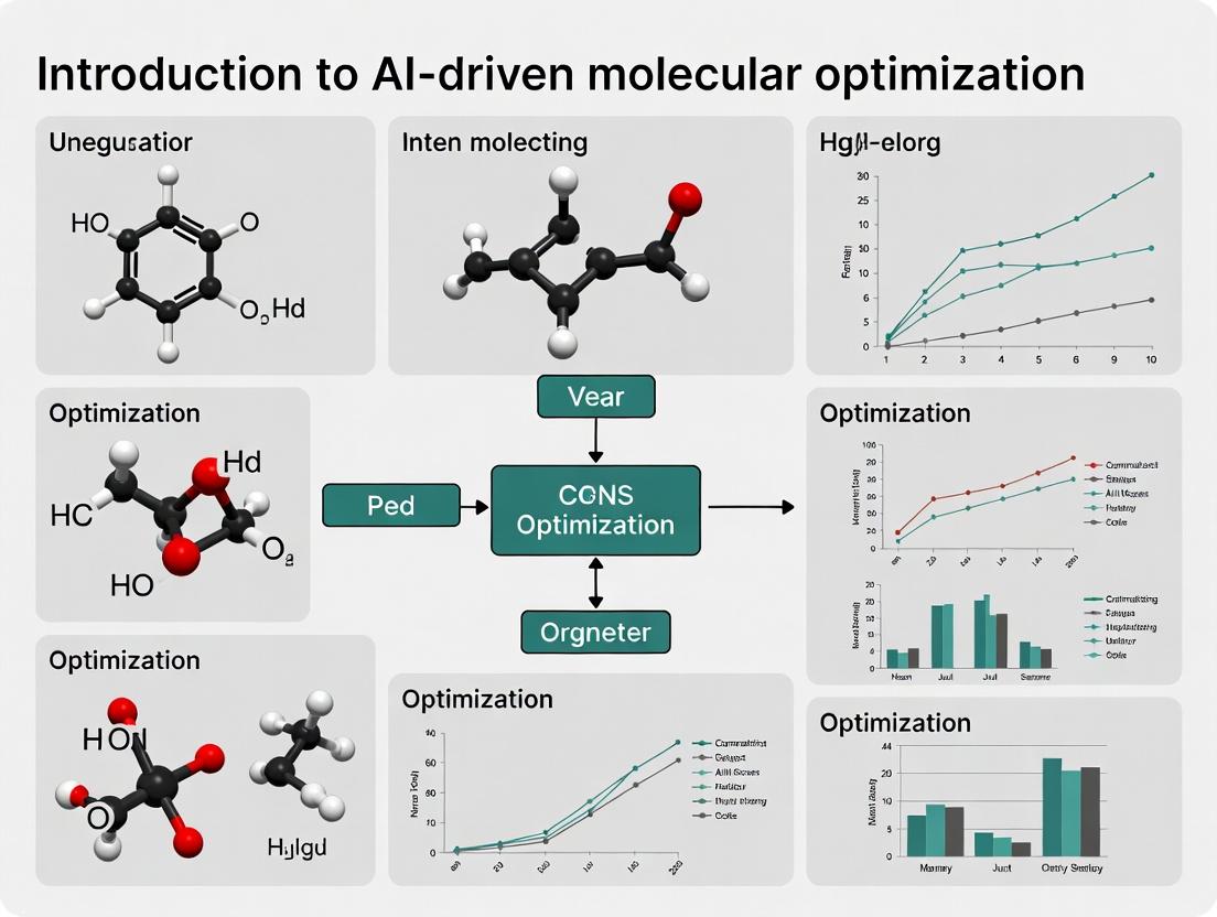
AI in Drug Discovery: A Practical Guide to Molecular Optimization for Scientists
This article provides a comprehensive overview of AI-driven molecular optimization for researchers and drug development professionals.
AI in Drug Discovery: A Practical Guide to Molecular Optimization for Scientists
Abstract
This article provides a comprehensive overview of AI-driven molecular optimization for researchers and drug development professionals. It explores the core principles, from defining objectives and navigating chemical space, to detailing key methodologies like generative models, reinforcement learning, and active learning. We address common challenges such as data scarcity, multi-property optimization, and explainability, while evaluating how these AI approaches compare to traditional methods in terms of speed, novelty, and success rates. The goal is to equip scientists with a practical understanding of how to implement and validate AI tools to accelerate the design of novel therapeutics with improved efficacy and safety profiles.
What is AI-Driven Molecular Optimization? Foundational Concepts for Researchers
Molecular optimization is the iterative, multi-parameter process of transforming a biologically active starting point (a "hit" or "lead" molecule) into a clinical candidate with the optimal balance of potency, selectivity, pharmacokinetic (PK), safety, and developability properties. Framed within the broader thesis of AI-driven molecular optimization research, this technical guide dissects the core challenge: navigating a vast, discrete, and constrained chemical space under conflicting objectives to arrive at viable drug molecules.
The Multi-Dimensional Optimization Problem
Drug discovery is not a singular objective problem. A potent binder to a target is useless if it cannot be synthesized, is rapidly metabolized, or is toxic. Molecular optimization requires simultaneous satisfaction of a dozen or more critical parameters, often with inherent trade-offs.
Table 1: Key Parameters in Molecular Optimization
| Parameter Category | Specific Metric | Typical Target/Constraint |
|---|---|---|
| Potency | IC50 / Ki | < 100 nM (often < 10 nM) |
| Selectivity | Ratio vs. anti-targets (e.g., hERG) | > 30-fold selectivity |
| Permeability | PAMPA, Caco-2, MDCK | Apparent Permeability (Papp) > 10 x 10⁻⁶ cm/s |
| Metabolic Stability | Microsomal/ Hepatocyte half-life (T½) | Human liver microsomal T½ > 30 min |
| CYP Inhibition | IC50 vs. CYP3A4, 2D6 | > 10 µM |
| Solubility | Kinetic/ Thermodynamic (pH 7.4) | > 100 µg/mL |
| Protein Binding | Fraction unbound (fu) | Species-dependent; influences PK/PD |
| In Vivo PK | Clearance (CL), Volume (Vd), Oral Bioavailability (F%) | Species-dependent; low CL, good F% desired |
| In Vitro Safety | hERG IC50, Ames Test, Cytotoxicity | hERG IC50 > 30 µM; Ames negative |
Core Methodologies and Experimental Protocols
Structure-Activity Relationship (SAR) Expansion
Objective: Systematically explore chemical space around a lead series to map the correlation between structural changes and biological activity. Protocol:
- Design: Using available structural data (target co-crystal, pharmacophore model), design analogues focusing on: a) Core scaffold modifications, b) Substituent exploration at R-groups, c) Bioisosteric replacement.
- Synthesis: Execute synthesis via parallel medicinal chemistry or automated synthesis platforms (e.g., Chemspeed, Vortex).
- Primary Screening: Test all compounds in a target-specific biochemical assay (e.g., FRET, TR-FRET, AlphaScreen). Run in 10-point dose-response, n=2, to determine IC50.
- Triaging: Compounds meeting the potency threshold (e.g., IC50 < 100 nM) advance to the In Vitro ADME panel.
2In VitroADME-Tox Profiling
Objective: Characterize the absorption, distribution, metabolism, excretion, and toxicity potential of lead candidates. Key Protocol: Metabolic Stability in Human Liver Microsomes (HLM):
- Reagent Prep: Thaw HLM (0.5 mg/mL final) in 100 mM phosphate buffer (pH 7.4). Prepare test compound (1 µM final) and NADPH regeneration system (1 mM NADP+, 5 mM G6P, 1 U/mL G6PDH).
- Incubation: Pre-incubate HLM + compound for 5 min at 37°C. Initiate reaction with NADPH system. Aliquot 50 µL at T = 0, 5, 15, 30, 45, 60 min into a stop solution (ACN with internal standard).
- Analysis: Centrifuge, dilute supernatant, and analyze via LC-MS/MS. Quantify peak area ratio (compound/IS) over time.
- Data Processing: Plot Ln(peak area ratio) vs. time. Calculate slope (k, min⁻¹). Half-life T½ = 0.693/k. Intrinsic Clearance (CLint) = (0.693/T½) * (mL incubation/mg microsomes).
The AI-Driven Optimization Paradigm
Modern approaches frame this as a computational search problem. The goal is to learn a function f(M) → P that maps a molecule M to a multi-dimensional profile P (potency, ADME, etc.) and use this to guide the search for the Pareto-optimal frontier.
Quantitative Structure-Activity Relationship (QSAR) Models
Workflow: Curated dataset → Molecular featurization (e.g., ECFP4 fingerprints, descriptors) → Model training (e.g., Random Forest, XGBoost, Neural Net) → Prediction for virtual library → Synthesis prioritization.
Title: QSAR Modeling and Virtual Screening Workflow
2De NovoMolecular Design with Generative AI
Generative models (VAEs, GANs, Transformers) learn the distribution of "drug-like" chemical space and generate novel structures conditioned on desired properties.
Title: AI-Driven De Novo Molecular Design Cycle
The Scientist's Toolkit: Key Research Reagent Solutions
Table 2: Essential Materials for Molecular Optimization Experiments
| Item | Function | Example/Supplier |
|---|---|---|
| Recombinant Target Protein | Biochemical assay substrate for potency screening. | Thermo Fisher, Sino Biological |
| Human Liver Microsomes (HLM) | In vitro system for predicting metabolic stability and metabolite identification. | Corning Life Sciences, Xenotech |
| Caco-2 Cell Line | Model for predicting intestinal permeability and efflux transporter effects (P-gp). | ATCC (HTB-37) |
| hERG-Expressing Cell Line | In vitro safety assay for cardiac liability risk assessment. | ChanTest (Kv11.1/HEK), Eurofins |
| LC-MS/MS System | Quantification of compounds in biological matrices for PK/ADME studies. | Sciex Triple Quad, Agilent Q-TOF |
| Automated Chemistry Platform | Enables high-throughput parallel synthesis for rapid SAR exploration. | Chemspeed Technologies, Unchained Labs |
| Molecular Featurization Software | Converts chemical structures into numerical descriptors for ML. | RDKit, MOE, Dragon |
| Generative Chemistry AI Platform | De novo design and multi-parameter optimization of molecules. | Exscientia, Insilico Medicine, Atomwise |
Defining molecular optimization as the core challenge underscores its complexity as a multi-objective, constrained search in a vast combinatorial space. The integration of high-throughput experimentation with AI-driven design and prediction represents a paradigm shift. The future lies in closed-loop systems where AI proposes molecules, robotics synthesizes them, and automated platforms test them, with data continuously feeding back to refine the AI models—accelerating the journey from hit to clinical candidate.
This whitepaper details the technical evolution of computational chemistry, framed within the broader thesis of AI-driven molecular optimization research. The journey from classical Quantitative Structure-Activity Relationship (QSAR) models to contemporary deep learning architectures represents a paradigm shift in how researchers predict molecular properties, design novel compounds, and accelerate the discovery pipeline. This guide provides an in-depth technical analysis for researchers and drug development professionals.
The QSAR Paradigm: Foundations and Methodology
Classical QSAR establishes mathematical relationships between a compound's physicochemical descriptors and its biological activity.
Core QSAR Equation: The fundamental Hansch equation is expressed as:
log(1/C) = k₁π + k₂σ + k₃Eₛ + k₄
Where C is the molar concentration producing a standard biological effect, π is hydrophobicity, σ is an electronic parameter, Eₛ is a steric parameter, and k are coefficients.
Experimental Protocol for Classical QSAR Development:
- Data Curation: Assay a congeneric series of molecules for a specific endpoint (e.g., IC₅₀).
- Descriptor Calculation: Compute physicochemical parameters (e.g., logP, molar refractivity, HOMO/LUMO energies) using software like DRAGON or MOE.
- Model Construction: Apply multivariate regression (MLR, PLS) using tools like SIMCA or in-house scripts.
- Validation: Employ leave-one-out (LOO) or leave-many-out (LMO) cross-validation. Assess using q² (cross-validated r²) and r² for the test set.
- Domain Applicability: Define the model's chemical space using leverage and standardization approaches.
Quantitative Data: Evolution of Model Performance
| Era | Typical Approach | Key Descriptors | Avg. Test Set r² (Reported Range) | Common Validation Method |
|---|---|---|---|---|
| 1970s-1980s | 2D Hansch Analysis | logP, σ, MR, Indicator Variables | 0.60 - 0.75 | LOO-CV |
| 1990s-2000s | 3D-QSAR (CoMFA, CoMSIA) | Steric/Electrostatic Fields, H-bonding | 0.65 - 0.80 | LOO-CV, Bootstrapping |
| 2000s-2010s | Machine Learning QSAR (RF, SVM) | Topological, Quantum Chemical (100s-1000s) | 0.70 - 0.85 | 5-Fold CV, Y-Randomization |
Title: Classical QSAR Model Development Workflow
The Rise of Machine Learning and Deep Learning
The transition to AI involves moving from hand-crafted descriptors to learned representations and from linear models to complex nonlinear approximators.
Key AI Model Architectures:
- Graph Neural Networks (GNNs): Treat molecules as graphs with atoms as nodes and bonds as edges. Message-passing mechanisms aggregate information to generate a molecular fingerprint (e.g., MPNN, GAT).
- Transformers: Adapted from NLP, these models process SMILES strings or molecular graphs using self-attention to capture long-range dependencies (e.g., ChemBERTa, Molecular Transformer).
- Generative Models: Variational Autoencoders (VAEs), Generative Adversarial Networks (GANs), and diffusion models learn the data distribution of molecules to generate novel, optimized structures.
Experimental Protocol for a Modern GNN Property Predictor:
- Dataset: Use a large, curated public dataset (e.g., ChEMBL, QM9). Apply stringent filtering for activity/measurement consistency.
- Data Splitting: Employ scaffold splitting (based on Bemis-Murcko scaffolds) to assess generalization, not random splitting.
- Model Implementation: Implement a message-passing neural network (MPNN) using PyTorch Geometric or DGL.
- Training: Use Adam optimizer, Mean Squared Error loss for regression, with early stopping on a validation set.
- Evaluation: Report RMSE, MAE, and R² on the held-out test set. Perform uncertainty quantification (e.g., deep ensembles, Monte Carlo dropout).
Quantitative Data: AI Model Performance Benchmarks
| Model Type | Dataset (Task) | Key Metric (Performance) | Hardware & Training Time | Reference Year |
|---|---|---|---|---|
| Random Forest | Tox21 (Classification) | Avg. ROC-AUC: 0.83 | CPU, ~1 hour | 2016 |
| MPNN | QM9 (HOMO Prediction) | MAE: ~43 meV | 1x GPU, ~1 day | 2017 |
| ChemBERTa | MoleculeNet (Multiple) | Avg. ROC-AUC: 0.80 | 4x GPU, ~1 week | 2021 |
| 3D GNN (SphereNet) | PDBBind (Affinity) | RMSE: 1.15 pKd | 1x GPU, ~2 days | 2022 |
AI-Driven Molecular Optimization: The New Frontier
This is the core of the thesis context: using AI not just for prediction, but for de novo design and iterative optimization.
Reinforcement Learning (RL) Protocol for Molecular Optimization:
- Agent: A generative model (e.g., RNN, Graph VAE).
- Environment: A scoring function (predictive model or simulator) that evaluates a generated molecule's properties (e.g., docking score, predicted bioactivity, ADMET).
- State: The current molecular structure (SMILES or graph).
- Action: A step in the generation process (e.g., adding an atom/bond, modifying a functional group).
- Reward: A composite score combining primary activity, synthetic accessibility (SA), and drug-likeness (QED).
- Training Loop: The agent generates molecules, receives rewards from the environment, and updates its policy (generation strategy) to maximize expected cumulative reward (e.g., via Policy Gradient or PPO).
Quantitative Data: Generative Model Output (Sample Benchmark)
| Optimization Goal | Generative Method | Starting Point | % Success (≥10uM & SA) | Notable Achieved Property Improvement |
|---|---|---|---|---|
| DRD2 Activity | REINVENT (RL) | Random | ~70% | >1000x pIC₅₀ increase in silico |
| JAK2 Inhibitors | GENTRL (VAE+RL) | Known Scaffold | N/A | Novel series designed & synthesized in <40 days |
| Optimize QED & SA | Graph MCTS | Any Molecule | ~95% | QED increase by 0.2-0.3 on average |
Title: Reinforcement Learning Loop for Molecular Design
The Scientist's Toolkit: Key Reagent Solutions
| Item / Solution | Function in AI-Driven Molecular Optimization | Example / Provider |
|---|---|---|
| RDKit | Open-source cheminformatics toolkit for descriptor calculation, fingerprinting, molecule manipulation, and SA scoring. | RDKit.org |
| PyTorch Geometric / DGL | Libraries for building and training Graph Neural Networks (GNNs) on molecular graph data. | PyG.org, DeepGraphLibrary.ai |
| DeepChem | High-level open-source framework wrapping ML models (TensorFlow/PyTorch) for drug discovery tasks. | DeepChem.io |
| Omega & ROCS (OpenEye) | Commercial software for generating biologically relevant 3D conformers and shape-based molecular alignment. | OpenEye Scientific |
| Schrödinger Suite | Integrated platform for computational chemistry, including force fields (FFLD), docking (Glide), and free-energy perturbation (FEP+). | Schrödinger |
| AutoDock-GPU / Vina | Open-source molecular docking software for high-throughput virtual screening and scoring. | Scripps Research |
| MOSES / GuacaMol | Benchmarking platforms with datasets, metrics, and baselines for evaluating generative models. | Publications: arXiv:1811.12823, arXiv:1905.13343 |
| Synthetic Accessibility (SA) Scorer | Algorithm to estimate the ease of synthesizing a proposed molecule (critical for reward function design). | Implemented in RDKit (based on SYLVIA) |
| Cloud/High-Performance Compute (HPC) | Essential for training large AI models and running massive virtual screens (e.g., AWS, Azure, Google Cloud). | NVIDIA DGX systems, Cloud GPU instances |
The systematic discovery and optimization of novel molecular entities, particularly for therapeutic applications, constitutes a fundamental challenge in chemical and pharmaceutical research. The thesis of modern AI-driven molecular optimization research posits that computational intelligence can radically accelerate this process, navigating the vast chemical space more efficiently than traditional methods. This guide examines the two dominant AI paradigms—classical Machine Learning (ML) and Deep Learning (DL)—that underpin this transformative shift, detailing their technical mechanisms, comparative performance, and practical implementation in molecular design.
Foundational Paradigms: Core Principles and Architectures
Classical Machine Learning in molecular design typically relies on curated feature engineering. Molecules are represented as fixed-length numerical vectors using descriptors (e.g., molecular weight, logP, topological torsion fingerprints) or learned fingerprints (e.g., ECFP). Algorithms such as Random Forest (RF), Support Vector Machines (SVM), and Gaussian Processes (GP) then model the relationship between these features and a target property (e.g., binding affinity, solubility).
Deep Learning utilizes hierarchical neural networks to automatically learn feature representations from raw or minimally preprocessed molecular inputs. Primary architectures include:
- Graph Neural Networks (GNNs): Directly operate on molecular graphs, with atoms as nodes and bonds as edges.
- Recurrent Neural Networks (RNNs) & Transformers: Process molecular string representations (e.g., SMILES, SELFIES).
- Generative Models: Variational Autoencoders (VAEs) and Generative Adversarial Networks (GANs) learn the underlying distribution of chemical structures to generate novel molecules.
Logical Relationship: ML vs. DL in Molecular Design Workflow
Title: Workflow Divergence Between ML and DL Paradigms
Quantitative Performance Comparison
Recent benchmark studies (2023-2024) on public datasets like MoleculeNet provide the following performance insights.
Table 1: Performance on Key Molecular Property Prediction Tasks (MAE/RMSE/ROC-AUC)
| Task (Dataset) | Metric | Best Classical ML (Model) | Best Deep Learning (Model) | Relative Improvement (DL vs. ML) | Data Size Requirement for DL Advantage |
|---|---|---|---|---|---|
| Solubility (ESOL) | RMSE (log mol/L) | 0.58 (Kernel Ridge) | 0.47 (Attentive FP GNN) | ~19% | > 1,000 samples |
| Drug Efficacy (Tox21) | ROC-AUC | 0.831 (Random Forest) | 0.855 (D-MPNN) | ~2.9% | > 5,000 samples |
| Quantum Property (QM9 - U₀) | MAE (kcal/mol) | ~0.50 (KRR w/ FCHL) | 0.08 (SphereNet) | ~84% | > 100k samples |
| Binding Affinity (PDBBind) | RMSE (pK) | 1.40 (RF on descriptors) | 1.15 (GNN-Geom) | ~18% | > 8,000 complexes |
Table 2: Generative Model Output for De Novo Design (2024 Benchmarks)
| Metric | Classical ML (Genetic Algorithm + SMILES) | Deep Learning (GPT-3.5 on SELFIES) | Deep Learning (cGNN VAE) |
|---|---|---|---|
| Validity (%) | 85% | 99.9% | 94% |
| Uniqueness (10k gen) | 65% | 82% | 92% |
| Novelty | High | Very High | High |
| Optimization Efficiency | Low | High | Medium |
| Compute Cost (GPU hrs) | < 10 | 50-100 | 150+ |
Experimental Protocols for Key Studies
Protocol A: Benchmarking Property Prediction with Random Forest vs. Graph Neural Network
- Objective: Compare predictive accuracy for aqueous solubility.
- Dataset: Curated ESOL dataset (~1,100 compounds).
- ML Protocol:
- Featurization: Compute 200-dimensional feature vector per molecule using RDKit descriptors (topological, constitutional, electronic).
- Model Training: Train a Scikit-learn Random Forest Regressor with 500 trees, max depth=15. Use an 80/20 train/test split with stratified sampling.
- Validation: 5-fold cross-validation on training set; final evaluation on held-out test set.
- DL Protocol:
- Featurization: Convert SMILES to molecular graph. Nodes: atom type, degree, hybridization. Edges: bond type, conjugation.
- Model Training: Train a DGL-LifeSci implemented MPNN (Message Passing Neural Network) with 3 message passing steps, hidden dim=128, and a global pooling readout.
- Validation: Same split as ML protocol. Use Adam optimizer (lr=0.001) with early stopping (patience=50 epochs).
Protocol B: Generative Molecular Design using a VAE
- Objective: Generate novel molecules with high predicted activity against a target (e.g., JAK2 kinase).
- Dataset: ChEMBL compounds with reported IC50 < 10 μM for JAK2 (approx. 2,500 molecules).
- Procedure:
- Data Preprocessing: Canonicalize SMILES, remove salts, apply molecular weight filter (200-500 Da). Convert to SELFIES representation for robust generation.
- Model Architecture: Build a VAE with:
- Encoder: 3-layer GRU RNN encoding SELFIES into a 256-dim latent vector (z).
- Decoder: Symmetric 3-layer GRU RNN reconstructing SELFIES from z.
- Property Predictor: A dense network on z, predicting pIC50.
- Training: Jointly train on reconstruction loss (cross-entropy), latent loss (KL divergence), and property prediction loss (MSE). Use teacher forcing.
- Generation & Optimization: Sample latent vectors from a Gaussian prior biased by the property predictor. Decode to generate novel SELFIES, which are then converted to molecules and filtered by SA score and synthetic accessibility.
The Scientist's Toolkit: Key Research Reagents & Solutions
Table 3: Essential Materials and Software for AI-Driven Molecular Design Experiments
| Item Name (Type) | Function/Benefit | Example Source/Package |
|---|---|---|
| RDKit (Cheminformatics Library) | Open-source toolkit for descriptor calculation, fingerprint generation, molecule manipulation, and visualization. Core for ML feature engineering. | rdkit.org |
| Mordred Descriptor Calculator | Calculates > 1,800 2D/3D molecular descriptors directly from SMILES, comprehensive for classical ML. | PyPI: mordred-descriptor |
| Deep Graph Library (DGL) or PyTorch Geometric (PyG) | Primary frameworks for building and training Graph Neural Networks (GNNs) on molecular graph data. | dgl.ai, pytorch-geometric.readthedocs.io |
| SELFIES (String Representation) | Robust, 100% valid molecular string representation for deep generative models, avoids SMILES syntax invalidity. | PyPI: selfies |
| GuacaMol / MOSES Benchmarks | Standardized benchmarks and datasets for evaluating generative model performance (novelty, diversity, etc.). | GitHub: BenevolentAI/guacamol |
| ADMET Prediction Models (e.g., ADMETlab) | Pre-trained models or webservices for early-stage pharmacokinetic and toxicity property filtering of generated molecules. | admetmesh.scbdd.com |
| GPU Computing Resource (e.g., NVIDIA A100) | Accelerates training of deep learning models, especially large GNNs and transformers, from days to hours. | Cloud providers (AWS, GCP, Azure) |
High-Level Experimental Workflow Diagram
Title: Integrated AI Molecular Design and Validation Pipeline
The choice between ML and DL is not hierarchical but contextual, dictated by the problem scope and resource constraints. Classical ML remains superior for small, high-quality datasets (< 1k samples), offering high interpretability, lower computational cost, and robust performance with well-engineered features. Deep Learning excels in capturing complex, non-linear structure-activity relationships from large, diverse datasets (> 10k samples) and is indispensable for de novo molecular generation. The ongoing thesis of AI-driven optimization research is increasingly synergistic, leveraging DL for feature discovery and generation, and robust ML models for final prediction and interpretation, thereby creating a hybrid pipeline that maximizes the strengths of both paradigms.
The pursuit of novel molecules with desired properties—be it for pharmaceuticals, materials, or agrochemicals—is fundamentally a search problem within a space of staggering vastness. The estimated number of synthetically accessible, drug-like molecules exceeds 10^60, a number dwarfing the count of stars in the observable universe. This vastness constitutes the chemical search space. Within the context of AI-driven molecular optimization research, the core challenge is to develop algorithms that can efficiently navigate this space to identify promising candidates, thereby accelerating discovery and reducing experimental costs. This guide examines the conceptual frameworks, quantitative dimensions, and computational methodologies essential for understanding and exploring this search space.
Quantifying the Chemical Search Space
The size and nature of the chemical search space are defined by combinatorial chemistry and the rules of chemical bonding. The following table summarizes key quantitative estimates.
Table 1: Quantitative Dimensions of the Chemical Search Space
| Metric | Estimated Value | Description & Source |
|---|---|---|
| Drug-like Molecules | 10^60 – 10^100 | Estimated number of organic molecules under 500 Da obeying Lipinski's rules and synthetic accessibility constraints (Polishchuk et al., J. Cheminform., 2013). |
| PubChem Compounds | ~114 million | Actual, synthesized, and registered small molecules in the PubChem database (2024 Live Search). |
| Enamine REAL Space | ~38 billion | Commercially accessible, make-on-demand compounds from Enamine's REAL (REadily AccessibLe) database (2024 Live Search). |
| Theoretical Organic Space (GDB) | 10^9 – 10^11 | Molecules in databases like GDB-17 (166 billion) enumerate possible structures within specific atom/rule limits (Reymond, Acc. Chem. Res., 2015). |
| Property Landscape Peaks | Variable, but sparse | The number of local maxima for a given property (e.g., binding affinity) is vastly smaller than the total space, creating a "needle-in-a-haystack" problem. |
Core Methodologies for Navigating the Search Space
AI-Driven Molecular Optimization Workflow
A standard AI-driven optimization cycle involves iterative proposal and evaluation.
Diagram 1: AI-Driven Molecular Optimization Cycle
Key Algorithmic Approaches
Experimental protocols for navigating the space rely on computational algorithms.
Protocol 1: De Novo Molecular Design with Reinforcement Learning (RL)
- Objective: To generate novel molecular structures optimizing a specific reward function (e.g., predicted binding affinity, QED).
- Methodology:
- Environment Setup: Define the action space (e.g., add an atom/bond, connect fragments) and state representation (e.g., molecular graph, SMILES string).
- Agent Model: Employ a deep neural network (e.g., RNN, Graph Neural Network) as the policy network.
- Reward Function: Design a composite reward (Rtotal = w1 * Rproperty + w2 * Rsyntheticaccessibility + w3 * R_novelty).
- Training: Use policy gradient methods (e.g., REINFORCE, PPO) to update the agent. The agent generates molecules (actions) and receives rewards from the environment (oracle).
- Sampling: After training, sample sequences of actions from the policy network to produce novel molecules.
- Key Reference: Zhou et al., Optimization of Molecules via Deep Reinforcement Learning, Sci. Rep., 2019.
Protocol 2: Bayesian Optimization for Molecular Property Prediction
- Objective: To find the global optimum of a black-box, expensive-to-evaluate function (e.g., experimental yield) with minimal evaluations.
- Methodology:
- Surrogate Model: Train a probabilistic model (typically a Gaussian Process) on an initial small dataset of molecules and their measured properties.
- Acquisition Function: Define a function (e.g., Expected Improvement, Upper Confidence Bound) that quantifies the potential utility of evaluating a new candidate.
- Iteration Loop: a) Find the molecule that maximizes the acquisition function based on the current surrogate model. b) Synthesize and test this molecule experimentally. c) Update the surrogate model with the new data point.
- Convergence: Repeat until a performance threshold is met or resources are exhausted.
- Key Reference: Griffiths & Hernández-Lobato, Constrained Bayesian Optimization for Automatic Chemical Design, arXiv, 2017.
The Scientist's Toolkit: Research Reagent Solutions
Table 2: Essential Materials & Tools for AI-Driven Molecular Optimization Research
| Item | Category | Function & Explanation |
|---|---|---|
| Enamine REAL Database | Compound Library | Provides a tangible, purchasable subset (~38B compounds) of the search space for virtual screening and validation of AI proposals. |
| RDKit | Open-Source Cheminformatics | A fundamental toolkit for manipulating molecular structures, calculating descriptors, and performing basic simulations. |
| Schrödinger Suite, OpenEye Toolkit | Commercial Software | Provides high-fidelity molecular docking, physics-based simulations (MD, FEP), and force fields for in silico evaluation. |
| AutoDock Vina, GNINA | Docking Software | Open-source tools for rapid, high-throughput virtual screening of AI-generated molecules against protein targets. |
| High-Throughput Screening (HTS) Assay Kits | Experimental Reagents | Enable parallel experimental validation of top AI-proposed candidates for activity, toxicity, or other properties. |
| DEL (DNA-Encoded Library) Technology | Synthesis & Screening | Allows the experimental synthesis and affinity-based screening of billions of compounds, providing massive empirical data for AI training. |
| Cloud Computing Credits (AWS, GCP, Azure) | Computational Infrastructure | Essential for training large AI models and running millions of molecular simulations/scoring operations. |
Mapping the Property Landscape
The relationship between chemical structure, representation, and property prediction is critical for effective navigation.
Diagram 2: From Chemical Space to Property Prediction
Understanding the chemical search space is not merely an academic exercise but a practical necessity for deploying AI in molecular optimization. The effective navigation of this space requires a synergistic combination of robust algorithmic strategies (RL, Bayesian optimization), accurate in silico evaluation tools, and targeted experimental validation. By quantifying the space, implementing rigorous computational protocols, and leveraging modern reagent and data resources, researchers can transform the problem from one of infinite possibility to one of tractable, intelligent discovery. The future of AI-driven research lies in creating tighter, more informed feedback loops between the virtual exploration of this vast space and real-world laboratory synthesis and testing.
In contemporary drug discovery, the central challenge is the simultaneous optimization of multiple, often competing, molecular properties. This multi-parameter optimization problem is a cornerstone of AI-driven molecular optimization research. The core objectives—potency (binding affinity to the target), selectivity (preference for the target over off-targets), favorable ADMET (Absorption, Distribution, Metabolism, Excretion, Toxicity) profiles, and synthesizability (feasibility of chemical synthesis)—represent a complex multidimensional landscape. AI and machine learning (ML) models are now essential for navigating this landscape, predicting properties, generating novel structures, and proposing optimization pathways that balance these critical objectives.
Deconstructing the Core Objectives
Quantitative Benchmarks and Target Profiles
Each objective has quantitative metrics that define success in early-stage research.
Table 1: Target Property Ranges for Oral Drug Candidates
| Property | Optimal Range/Target | Measurement Assay |
|---|---|---|
| Potency (IC50/Ki) | < 100 nM | Enzyme inhibition, Cell-based efficacy |
| Selectivity Index | > 30x (vs. primary off-targets) | Counter-screening panels |
| Lipophilicity (cLogP) | 1-3 | Computational prediction, HPLC |
| Permeability (Caco-2 Papp) | > 20 x 10⁻⁶ cm/s | Caco-2 assay |
| Microsomal Stability (Clint) | < 30 μL/min/mg | Human liver microsome assay |
| hERG Inhibition (IC50) | > 10 μM | Patch-clamp, binding assay |
| Aqueous Solubility (PBS) | > 100 μg/mL | Kinetic solubility assay |
| Synthesizability (SA Score) | < 4.5 | Synthetic Accessibility Score |
Interdependencies and Trade-offs
Key trade-offs exist between these objectives. High potency is often achieved by increasing lipophilicity, which can negatively impact solubility, metabolic stability, and increase hERG risk. Improving metabolic stability via steric blocking can increase molecular weight, harming permeability. AI models are trained to recognize these non-linear relationships.
Diagram 1: Key trade-offs in multi-parameter optimization
AI-Driven Methodologies for Balanced Optimization
Predictive Model Pipelines
AI integrates data from diverse assays to build predictive Quantitative Structure-Property Relationship (QSPR) models.
Experimental Protocol 1: High-Throughput ADMET Profiling for Model Training
- Library Preparation: Curate a diverse chemical library (500-2000 compounds) spanning lead-like space.
- Parallel Assay Execution:
- Solubility: Use nephelometry in phosphate buffer (pH 7.4).
- Metabolic Stability: Incubate compounds (1 μM) with human liver microsomes (0.5 mg/mL). Quantify parent compound loss via LC-MS/MS at 0, 5, 15, 30, 45 min.
- Permeability: Conduct Caco-2 assay in 24-well transwell plates. Measure apparent permeability (Papp) in A-B and B-A directions.
- CYP Inhibition: Fluorescent probe assays for CYP3A4, 2D6, 2C9.
- Data Curation: Normalize all readouts to internal controls. Apply strict quality control (QC) flags.
- Model Training: Use molecular fingerprints (ECFP) or graph representations as features. Train Random Forest or Gradient Boosting models for each ADMET endpoint. Validate via 5-fold cross-validation.
Multi-Objective Optimization Algorithms
AI optimizers search chemical space for molecules satisfying multiple criteria.
- Multi-Objective Reinforcement Learning (MORL): An agent generates molecules (action) and receives a vector reward [PotencyScore, SelectivityScore, ADMET_Score].
- Pareto Optimization: Identifies molecules where improving one objective worsens another (Pareto front).
- Conditional Generative Models: Models like Conditional Variational Autoencoders (CVAE) generate molecules conditioned on desired property ranges.
Diagram 2: Closed-loop AI optimization workflow
The Scientist's Toolkit: Research Reagent Solutions
Table 2: Essential Reagents & Kits for Core Objective Profiling
| Item | Function | Example Vendor/Product |
|---|---|---|
| Recombinant Target Protein & Isoforms | For potency & selectivity binding assays. | Eurofins, BPS Bioscience |
| Phospholipid Vesicles (PAMPA) | High-throughput prediction of passive permeability. | Pion Inc. PAMPA Evolution |
| Pooled Human Liver Microsomes (HLM) | In vitro assessment of metabolic stability (Phase I). | Corning Gentest, XenoTech |
| Cryopreserved Human Hepatocytes | Integrated assessment of metabolism & toxicity (Phase I/II). | BioIVT, Lonza |
| hERG Expressing Cell Line | Screening for cardiac ion channel liability. | Charles River, Eurofins |
| Caco-2 Cell Line | Gold-standard assay for intestinal permeability & efflux. | ATCC, Sigma-Aldrich |
| CYP450 Isozyme Kits | Profiling inhibition of key metabolic enzymes. | Promega P450-Glo, Thermo Fisher |
| Kinetic Solubility Assay Kit | Rapid measurement of aqueous solubility. | Cyprotex Solubility Kit |
| Click Chemistry Toolkit | For rapid late-stage functionalization to improve properties. | Sigma-Aldrich, J&K Scientific |
Integrated Protocol for Tiered Profiling
Experimental Protocol 2: Tiered In Vitro Profiling of AI-Designed Hits
- Tier 1 (Primary):
- Potency: Dose-response in primary target assay (n=3, 10-point dilution).
- Selectivity: Screen at 10 μM against 3-5 closest orthologs/isoforms.
- ClogP/Solubility: Computational prediction + experimental kinetic solubility.
- Tier 2 (Secondary ADMET):
- Microsomal Stability: Incubate at 1 μM with HLM. Calculate intrinsic clearance (Clint).
- PAMPA Permeability: Assess passive diffusion.
- CYP Inhibition: Screen at 10 μM against CYP3A4, 2D6.
- Tier 3 (Advanced):
- Full CYP Panel: IC50 determination for inhibiting CYPs.
- hERG Patch Clamp: IC50 determination on hERG-expressing cells.
- Cytotoxicity: Assess in HepG2 cells (48h exposure).
- Synthesizability Assessment:
- Retrosynthesis: Use AI tool (e.g., ASKCOS, IBM RXN) to propose routes.
- Complexity Scoring: Calculate SA Score, ring complexity, chiral centers.
- Medicinal Chemistry Review: Expert evaluation of proposed syntheses.
Data Integration and Decision Making
Final candidate selection requires weighted integration of all data.
Table 3: Hypothetical AI-Optimized Compound Series Profile
| Property | Lead A | Lead B (AI-Optimized) | Target |
|---|---|---|---|
| Target IC50 (nM) | 12 | 25 | < 100 |
| Selectivity (Fold vs. Off-target X) | 5 | 45 | > 30 |
| cLogP | 4.2 | 2.8 | 1-3 |
| Microsomal Clint (μL/min/mg) | 45 | 18 | < 30 |
| hERG IC50 (μM) | 8 | >30 | > 10 |
| Papp (10⁻⁶ cm/s) | 15 | 22 | > 20 |
| SA Score | 3.2 | 4.1 | < 4.5 |
| Synthetic Steps (longest linear sequence) | 9 | 6 | Minimize |
The data demonstrates a classic optimization: Lead B accepts a modest reduction in absolute potency to achieve marked improvements in selectivity, ADMET profile, and synthetic simplicity, representing a more balanced and developable candidate—a outcome efficiently identified by AI-driven Pareto analysis.
Balancing potency, selectivity, ADMET, and synthesizability is no longer a purely empirical, sequential process. Within the thesis of AI-driven molecular optimization, it is a unified computational-experimental feedback cycle. AI models predict complex property trade-offs, generative algorithms propose novel chemical matter navigating this multi-objective landscape, and focused experimental protocols validate the predictions. This integrated, data-driven approach significantly de-risks the path from hit identification to preclinical candidate, accelerating the delivery of safer, more effective therapeutics.
How AI Optimizes Molecules: Key Algorithms and Real-World Applications
The pursuit of novel molecular entities with desired properties is a cornerstone of modern chemistry and drug discovery. Within the broader thesis of AI-driven molecular optimization research, de novo molecular design represents a paradigm shift from virtual screening of known libraries to the generative construction of entirely new, synthetically accessible, and property-optimized chemical structures. Generative models, including Variational Autoencoders (VAEs), Generative Adversarial Networks (GANs), and Transformers, have emerged as powerful engines for this task, each with distinct architectures and learning principles enabling the exploration of vast, uncharted chemical space.
Core Generative Architectures: Mechanisms and Applications
Variational Autoencoders (VAEs)
VAEs learn a continuous, structured latent representation of molecular data (often SMILES strings or graphs). The encoder compresses an input molecule into a probability distribution in latent space, typically a Gaussian. A point sampled from this distribution is then decoded to reconstruct the original molecule or generate a novel one. This continuous space allows for smooth interpolation and optimization via gradient-based methods.
Key Experiment Protocol (Character VAE for SMILES Generation):
- Data Preparation: Curate a dataset of valid SMILES strings (e.g., from ZINC or ChEMBL). Implement SMILES tokenization (character or atom-level).
- Model Architecture: Define an encoder (e.g., bidirectional GRU or 1D CNN) that outputs parameters (μ, σ) for the latent Gaussian distribution. Define a decoder (e.g., GRU) to reconstruct the token sequence from a latent vector
z, sampled using the reparameterization trick:z = μ + σ * ε, whereε ~ N(0,1). - Training: Minimize the loss function:
Loss = Reconstruction Loss (Cross-Entropy) + β * KL Divergence Loss, where KL loss regularizes the latent space. The β parameter controls the trade-off between reconstruction accuracy and latent space regularity. - Generation: Sample a random vector
zfrom the prior distributionN(0, I)and pass it through the decoder to generate a novel SMILES string.
Generative Adversarial Networks (GANs)
GANs frame generation as an adversarial game between a Generator (G) and a Discriminator (D). G learns to map random noise to realistic molecular structures, while D learns to distinguish real molecules from generated ones. Through this competition, G improves its output to fool D.
Key Experiment Protocol (Organizational GAN for Molecular Graphs):
- Data Preparation: Represent molecules as graphs with node (atom) and edge (bond) features.
- Model Architecture: The generator (
G) is typically a multi-layer perceptron (MLP) that outputs a probabilistic graph (node and edge existence probabilities). The discriminator (D) is a graph neural network (GNN) that classifies graphs as real or generated. - Training: Alternate between:
- Training D: Maximize
log(D(real_molecule)) + log(1 - D(G(random_noise))). - Training G: Minimize
log(1 - D(G(random_noise)))or maximizelog(D(G(random_noise))).
- Training D: Maximize
- Generation: Input a random noise vector to the trained generator to produce a probabilistic graph, which is then discretized (e.g., using argmax or sampling) to yield a molecular graph.
Transformers
Originally designed for sequence transduction, Transformers have been adapted for molecular generation by treating SMILES or SELFIES strings as sequences and learning to predict the next token in an autoregressive manner. They excel at capturing long-range dependencies within the molecular representation.
Key Experiment Protocol (Transformer-based Autoregressive Generation):
- Data Preparation: Tokenize SMILES/SELFIES strings into subword units using algorithms like BPE (Byte Pair Encoding).
- Model Architecture: Utilize a standard Transformer decoder stack (or encoder-decoder) with masked self-attention. The model takes a sequence of tokens and predicts the next token at each position.
- Training: Train using teacher forcing to minimize the negative log-likelihood of the target sequence (the molecule itself).
- Generation: Perform autoregressive sampling (e.g., nucleus sampling or beam search) starting from a start token (
[CLS]or<s>) to generate a novel token sequence until an end token is produced.
Comparative Performance Analysis
Table 1: Quantitative Comparison of Generative Model Performance on Benchmark Tasks (e.g., Guacamol, MOSES)
| Metric | VAE (Character) | GAN (Graph-based) | Transformer (SELFIES) | Notes / Source |
|---|---|---|---|---|
| Validity (%) | 94.2% | 98.5% | 99.7% | Proportion of generated strings that correspond to valid molecules. SELFIES guarantees 100% syntax validity. |
| Uniqueness (%) | 87.4% | 91.1% | 95.8% | Proportion of unique molecules among a large set of valid generated molecules. |
| Novelty (%) | 92.3% | 89.5% | 96.2% | Proportion of valid, unique molecules not present in the training set. |
| Reconstruction Rate (%) | 76.5% | 61.2% (Graph Match) | 84.3% | Ability to accurately reconstruct a held-out test set molecule from its latent code/seed. |
| Diversity (FCD/MMD) | 0.89 (FCD) | 0.92 (FCD) | 0.95 (FCD) | Frechet ChemNet Distance or MMD; lower is better for FCD, higher for diversity metrics. |
| Optimization Success Rate | 75% | 68% | 82% | Success in generating molecules meeting specific property targets (e.g., QED, SAS). |
Data synthesized from recent benchmark studies (2023-2024) on Guacamol and MOSES datasets, including results from models like ChemVAE, MolGAN, and Chemformer.
The Scientist's Toolkit: Essential Research Reagents & Solutions
Table 2: Key Software Libraries and Resources for De Novo Molecular Design
| Item Name | Category | Primary Function | Typical Use Case |
|---|---|---|---|
| RDKit | Cheminformatics Library | Manipulation and analysis of chemical structures, descriptor calculation, and fingerprint generation. | Converting SMILES to mol objects, calculating molecular properties (e.g., LogP, TPSA), generating Morgan fingerprints. |
| DeepChem | Deep Learning Library | Provides high-level APIs for molecular machine learning, including dataset handling, model layers, and metrics. | Building and training Graph Neural Networks (GNNs) for property prediction within a generative pipeline. |
| PyTorch / TensorFlow | Deep Learning Framework | Low-level tensor operations and automatic differentiation for building and training custom neural network architectures. | Implementing the core components of VAEs, GANs, or Transformers (encoders, decoders, generators, discriminators). |
| Guacamol / MOSES | Benchmarking Suite | Standardized benchmarks and datasets for evaluating generative models on metrics like validity, novelty, and property optimization. | Comparing the performance of a newly developed generative model against published baselines. |
| SELFIES | Molecular Representation | A 100% robust string-based molecular representation that guarantees syntactic and semantic validity. | Used as the input/output alphabet for Transformer or VAE models to avoid invalid SMILES generation. |
| Open Babel / ChemAxon | Cheminformatics Platform | Format conversion, descriptor calculation, and high-throughput molecular processing. | Preparing large datasets, standardizing tautomers, or performing vendor catalogue screening post-generation. |
Key Methodological Workflows
Title: VAE Training and Generation Workflow
Title: Adversarial Training Cycle for Molecular GANs
Title: Autoregressive Molecular Generation with Transformers
Within the broader thesis of Introduction to AI-driven molecular optimization research, reframing traditional optimization tasks as sequential decision problems is a paradigm shift. This approach, powered by Reinforcement Learning (RL), is revolutionizing the design of novel molecules with desired properties, a core challenge in modern drug discovery.
The Sequential Decision-Making Framework
In molecular optimization, the goal is to iteratively modify a molecular structure to improve a target property (e.g., binding affinity, solubility, synthetic accessibility). RL frames this as a Markov Decision Process (MDP):
- State (s): A representation of the current molecule (e.g., SMILES string, molecular graph, fingerprint).
- Action (a): A modification to the molecular structure (e.g., adding a functional group, changing a bond, attaching a fragment).
- Reward (r): A numerical score evaluating the quality of the new molecule after the action. This often combines primary objectives (druggability score) with penalties for undesirable properties.
- Policy (π): The AI agent's strategy—a function that selects the next chemical action given the current molecular state.
The agent learns an optimal policy through exploration and exploitation, maximizing the cumulative reward (e.g., the property of the final molecule in a sequence of modifications).
Key Methodologies and Experimental Protocols
Deep Q-Networks (DQN) for Discrete Action Spaces
This protocol trains an agent to predict the value of possible molecular modifications.
Protocol:
- Environment Setup: Define the chemical space (e.g., a set of permitted fragments and reactions) and the property prediction model (the "oracle").
- Replay Buffer Initialization: Create a memory store for past experiences (state, action, reward, next state).
- Network Architecture: Implement two neural networks: a Q-network (parameters θ) and a target network (parameters θ⁻). The input is the molecular state representation; the output is a Q-value for each possible action.
- Training Loop: a. Initialize a starting molecule (state s). b. Select an action a via an ε-greedy policy based on the Q-network's predictions. c. Execute the action in the chemical environment, generating a new molecule (state s') and receiving a reward r. d. Store the experience (s, a, r, s') in the replay buffer. e. Sample a random batch of experiences from the buffer. f. Compute the target Q-value: y = r + γ * maxₐ' Q(s', a'; θ⁻). g. Update the Q-network parameters by minimizing the Mean Squared Error loss between Q(s, a; θ) and y. h. Periodically update the target network: θ⁻ ← τθ + (1-τ)θ⁻.
- Evaluation: Use the trained policy to generate novel molecules from seed compounds, ranking them by predicted cumulative reward.
Policy Gradient (e.g., REINFORCE) for Generative Models
This protocol directly optimizes a stochastic policy, often a generative model that produces molecules token-by-token (like a SMILES string).
Protocol:
- Policy Model: Define a parameterized policy πθ (a Recurrent Neural Network or Transformer) that outputs a probability distribution over the next chemical token/action given the sequence so far.
- Episode Generation: Use the current policy πθ to sample complete sequences of actions, generating a batch of N molecules.
- Reward Calculation: Score each generated molecule i using the reward function Rᵢ (e.g., a weighted sum of quantitative estimate of drug-likeness (QED) and synthetic accessibility score (SAS)).
- Gradient Estimation: Compute the gradient to maximize the expected reward: ∇θ J(θ) ≈ (1/N) Σᵢ₌₁ᴺ Rᵢ ∇θ log πθ(sequenceᵢ).
- Policy Update: Adjust the policy parameters θ in the direction of the gradient using stochastic gradient ascent.
- Iteration: Repeat steps 2-5 until convergence, resulting in a policy biased toward generating high-reward molecules.
Quantitative Performance Data
Table 1: Comparison of RL Frameworks in Molecular Optimization (Benchmark: Guacamol)
| RL Algorithm | Benchmark (Guacamol Score) | Avg. Top-1 Property Improvement | Computational Cost (GPU days) | Sample Efficiency (Molecules) |
|---|---|---|---|---|
| DQN (Zhou et al., 2019) | 0.84 | 38% (QED) | ~7 | ~50,000 |
| Policy Gradient (REINFORCE) | 0.79 | 42% (DRD2 Activity) | ~5 | ~100,000 |
| Proximal Policy Optimization (PPO) | 0.91 | 51% (Multi-Objective) | ~12 | ~25,000 |
| Actor-Critic with Experience Replay | 0.87 | 47% (LogP) | ~10 | ~15,000 |
Table 2: Key Molecular Properties Targeted by RL Optimization
| Property | Typical Reward Function Component | Measurement Method | Optimization Goal |
|---|---|---|---|
| Quantitative Estimate of Drug-likeness (QED) | 0.0 to 1.0 | Calculated from descriptors | Maximize (Closer to 1.0) |
| Synthetic Accessibility Score (SAS) | 1.0 (Easy) to 10.0 (Hard) | Fragment-based complexity | Minimize (Closer to 1.0) |
| Binding Affinity (pIC50 / ΔG) | Negative log of IC50 or ΔG | In silico docking (e.g., AutoDock Vina) | Maximize (More Negative ΔG) |
| Octanol-Water Partition Coeff. (LogP) | Target range (e.g., 2.0 - 3.0) | Computational estimation (e.g., XLogP) | Penalize deviation from range |
| Pharmacokinetic/Toxicity Risk | Binary or continuous score | ADMET prediction models (e.g., SMARTS alerts) | Minimize risk |
Visualization of the RL Optimization Cycle
Diagram 1: The Molecular RL Agent-Environment Interaction Loop
Diagram 2: End-to-End RL Molecular Optimization Workflow
The Scientist's Toolkit: Key Research Reagent Solutions
Table 3: Essential Tools for AI-Driven Molecular Optimization Research
| Tool / Reagent Category | Specific Example(s) | Function in the Research Pipeline |
|---|---|---|
| Chemical Representation Library | RDKit, DeepChem | Converts molecules to graphs, fingerprints, or descriptors for model input. |
| RL Algorithm Framework | OpenAI Gym, Stable-Baselines3, RLlib | Provides standardized environments and implementations of DQN, PPO, SAC, etc. |
| Deep Learning Platform | PyTorch, TensorFlow, JAX | Enables building and training policy and value networks. |
| Property Prediction Oracle | Commercial: Schrodinger, OpenEye. Open-source: AutoDock Vina, QSAR models. | Provides the reward signal by predicting molecular properties or binding affinities. |
| Molecular Generation Environment | GuacaMol, MolGym, ChemRL | Benchmark suites and customizable environments for developing RL agents. |
| High-Performance Computing (HPC) | GPU clusters (NVIDIA), Cloud compute (AWS, GCP) | Accelerates the intensive training of RL models and molecular simulations. |
| Chemical Database | ZINC, PubChem, ChEMBL | Sources of seed molecules and training data for pre-training or auxiliary tasks. |
| Synthesis Planning Software | AiZynthFinder, ASKCOS, Reaxys | Validates the synthetic feasibility of AI-generated molecules (post-RL filtering). |
1. Introduction within an AI-Driven Molecular Optimization Thesis
The pursuit of novel molecules with desired properties—be it high binding affinity, specific enzymatic activity, or optimal pharmacokinetics—is a cornerstone of modern research. This chapter of our thesis on Introduction to AI-driven molecular optimization research addresses the critical bottleneck of experimental efficiency. Traditional high-throughput screening (HTS) is often resource-intensive and explores chemical space naively. Active Learning (AL) and Bayesian Optimization (BO) form a synergistic computational framework that intelligently selects the most informative experiments to perform next, creating a closed-loop, AI-driven cycle for rapid molecular optimization.
2. Core Theoretical Framework
- Active Learning (AL): A machine learning paradigm where the algorithm proactively queries an "oracle" (e.g., a wet-lab experiment or a high-fidelity simulation) for labels of the most uncertain or informative data points. The goal is to maximize performance with minimal data.
- Bayesian Optimization (BO): A probabilistic strategy for finding the global optimum (e.g., highest activity) of a black-box, expensive-to-evaluate function. It combines a surrogate model (typically a Gaussian Process, GP) to approximate the objective function and an acquisition function to decide the next point to evaluate by balancing exploration (high uncertainty) and exploitation (high predicted value).
The integration forms a powerful cycle: the GP model quantifies prediction and uncertainty across the molecular design space; the acquisition function, acting as the AL query strategy, selects the candidate(s) predicted to yield the maximum information gain or performance improvement; these candidates are synthesized and tested experimentally; and the new data is used to update the model, closing the loop.
Table 1: Comparison of Common Acquisition Functions in Bayesian Optimization
| Acquisition Function | Key Formula/Principle | Best For | Exploration/Exploitation Balance |
|---|---|---|---|
| Expected Improvement (EI) | ( EI(x) = \mathbb{E}[\max(f(x) - f(x^+), 0)] ) | General-purpose optimization, finding global maxima. | Adaptive, based on improvement probability. |
| Upper Confidence Bound (UCB) | ( UCB(x) = \mu(x) + \kappa \sigma(x) ) | Tunable trade-off via ( \kappa ). | Explicitly controlled by ( \kappa ) parameter. |
| Probability of Improvement (PI) | ( PI(x) = \Phi\left(\frac{\mu(x) - f(x^+)}{\sigma(x)}\right) ) | Local optimization, rapid initial gains. | Tends to be more exploitative. |
| Knowledge Gradient (KG) | Considers optimal posterior mean after evaluation. | Noisy functions, sequential batch design. | Considers full information value. |
3. Detailed Experimental Protocol for an AL/BO-Driven Molecular Design Cycle
Protocol: Closed-Loop Optimization of a Lead Compound Series
Objective: Maximize the target binding affinity (pIC50) of a chemical series over 5 iterative cycles, starting from an initial dataset of 50 compounds.
Step 1: Initial Library Design & Data Generation
- Design an initial diverse set of 50 molecules using a fragment-based or scaffold-hopping approach.
- Synthesis & Assay: Synthesize compounds via automated parallel chemistry. Measure pIC50 using a standardized biochemical binding assay (e.g., fluorescence polarization). This forms the seed dataset ( D{0} = { (xi, yi) }{i=1}^{50} ).
Step 2: Molecular Representation (Featurization)
- Convert SMILES strings of each molecule ( x_i ) into numerical feature vectors. Common methods include:
- Extended-Connectivity Fingerprints (ECFPs): 2048-bit radius-2 fingerprints.
- Molecular Descriptors: RDKit-calculated descriptors (e.g., MolWt, LogP, TPSA, number of rotatable bonds).
- Learned Representations: Pre-trained molecular transformer embeddings (e.g., from ChemBERTa).
Step 3: Surrogate Model Training
- Train a Gaussian Process (GP) regression model on ( D_{t} ) (where ( t ) is the current cycle).
- Kernel Selection: Use a Matérn 5/2 kernel to model the objective function. Optimize kernel hyperparameters (length scales, noise variance) by maximizing the log marginal likelihood.
- The GP provides a predictive mean ( \mu(x) ) and uncertainty ( \sigma(x) ) for any candidate molecule ( x ).
Step 4: Candidate Selection via Acquisition Function
- Calculate the acquisition function ( \alpha(x) ) (e.g., Expected Improvement) for all molecules in a pre-enumerated virtual library (e.g., 10,000 analogs generated via defined reaction rules).
- Select the top ( n ) candidates (( n = 5 ) for batch mode) that maximize ( \alpha(x) ). For batch selection, use a diversity-promoting method like K-means clustering on the feature space of the top 100 scorers, then pick the highest-( \alpha ) candidate from each cluster.
Step 5: Experimental Validation & Loop Closure
- Synthesize and assay the ( n ) selected candidates as in Step 1.
- Augment the dataset: ( D{t+1} = D{t} \cup { (x{new}, y{new}) } ).
- Repeat from Step 3 for a predefined number of cycles or until a performance target (e.g., pIC50 > 8.0) is met.
4. Visualizing the Workflow and Molecular Representations
Diagram 1: Closed-loop AL/BO cycle for molecular optimization.
Diagram 2: Pathways from SMILES to model-ready features.
5. The Scientist's Toolkit: Key Research Reagent Solutions
Table 2: Essential Materials for an AI-Guided Molecular Optimization Campaign
| Item/Category | Example Product/System | Function in the Workflow |
|---|---|---|
| Chemical Synthesis | ChemSpeed or Biotage Automated Synthesizers | Enables rapid, parallel synthesis of AL/BO-selected compound candidates. |
| Assay Kit | Cisbio HTRF or Thermo Fisher FP Binding Assay Kits | Provides standardized, high-throughput biochemical assays for quantitative activity measurement (pIC50). |
| Molecular Featurization | RDKit Open-Source Toolkit | Generates fingerprints (ECFPs) and molecular descriptors from SMILES. |
| Surrogate Modeling | GPyTorch or scikit-learn Python Libraries | Builds and trains Gaussian Process regression models on experimental data. |
| Bayesian Optimization | BoTorch or Ax Platform | Provides state-of-the-art implementations of acquisition functions and batch optimization loops. |
| Virtual Library | Enamine REAL or WuXi GalaXi Space | Provides access to ultra-large, synthesizable virtual compounds for candidate selection. |
| Data Management | CDD Vault or Benchling ELN | Securely manages experimental data, structures, and results for seamless integration with AI models. |
In AI-driven molecular optimization research, the primary objective is to guide the iterative design of novel compounds with enhanced properties, such as drug efficacy or binding affinity. The foundational challenge is how to represent a molecule for computational analysis. The choice of representation directly dictates which machine learning architectures can be used, what information is preserved or lost, and ultimately, the success of the optimization campaign. This whitepaper provides an in-depth technical guide to the three dominant paradigms: SMILES strings, molecular graphs, and 3D representations, detailing their implementation, trade-offs, and experimental protocols for their use in modern AI models.
Technical Deep Dive: Core Representations
SMILES (Simplified Molecular-Input Line-Entry System)
SMILES is a line notation encoding molecular structure as an ASCII string using a depth-first traversal of the molecular graph. It is compact and human-readable but presents challenges due to its non-uniqueness (multiple SMILES can represent the same molecule) and syntactic sensitivity.
Key AI Application: Sequence-based models (RNNs, Transformers). Models like ChemBERTa are pre-trained on large SMILES corpora to learn chemical language.
Limitation: The string representation does not explicitly encode molecular symmetry or complex spatial relationships.
Molecular Graph Representation
A molecule is represented as an undirected graph G = (V, E), where atoms are nodes (V) and bonds are edges (E). Node and edge features encode atom/bond types, charges, etc.
Key AI Application: Graph Neural Networks (GNNs). Models like Message Passing Neural Networks (MPNNs) and Graph Attention Networks (GATs) operate directly on this structure, aggregating neighbor information to learn molecular fingerprints.
Advantage: Inherently captures topological structure and is invariant to atom indexing.
3D (Geometric) Representation
This representation includes the spatial coordinates of each atom, defining the molecular conformation. It may also include quantum chemical properties (partial charges, orbital information).
Key AI Application: Geometric Deep Learning (GDL). Models like SchNet, SE(3)-Transformers, and Equivariant GNNs are designed to be rotationally and translationally invariant (or equivariant), crucial for predicting properties dependent on 3D geometry, such as molecular energy or protein-ligand binding poses.
Advantage: Essential for modeling quantum mechanical properties and intermolecular interactions.
Quantitative Comparison of Representations
The performance of representations varies significantly across benchmark tasks. The following table summarizes recent findings (2023-2024) from key literature, including datasets like QM9, MoleculeNet, and PDBbind.
Table 1: Performance Benchmark of AI Models Using Different Molecular Representations
| Representation | Model Archetype | Sample Benchmark (Dataset) | Key Metric Result | Primary Strength | Primary Weakness |
|---|---|---|---|---|---|
| SMILES | Transformer (Chemformer) | MoleculeNet (Clintox) | ROC-AUC: 0.936 | High-throughput generation, simplicity | Poor capture of spatial & topological rules |
| 2D Graph | GNN (MPNN) | MoleculeNet (FreeSolv) | RMSE: 1.02 kcal/mol | Excellent topology capture, invariant | No explicit 3D geometry |
| 3D Graph | Equivariant GNN (PaiNN) | QM9 (μ) | MAE: 0.012 D | Quantum property accuracy, geometric reasoning | Computationally intensive, requires conformers |
| 3D Surface | 3D CNN | PDBbind (Core Set) | RMSD: 1.45 Å (Pose Prediction) | Directly models interaction surfaces | Very high computational cost |
| Hybrid (Graph+3D) | Multi-modal Transformer | QM9 (α) | MAE: 0.046 Bohr³ | Balances efficiency and geometric fidelity | Model complexity, integration challenges |
Experimental Protocols for Key Studies
Protocol: Training a SMILES-Based Transformer forDe NovoMolecular Generation
- Data Curation: Assemble a dataset of validated SMILES strings (e.g., from ChEMBL >1 million compounds). Canonicalize all SMILES using RDKit.
- Tokenization: Implement Byte Pair Encoding (BPE) or atom-level tokenization to create a vocabulary.
- Model Architecture: Configure a standard Transformer decoder-only architecture (e.g., 8 layers, 8 attention heads, 512 embedding dimension).
- Training: Use a causal language modeling objective (next-token prediction). Optimize with AdamW (lr=1e-4), batch size 128, for ~50 epochs.
- Generation: Use nucleus sampling (top-p=0.9) to generate novel SMILES strings from a seed fragment.
- Validation: Pass generated SMILES through RDKit for chemical validity checks and property prediction.
Protocol: Training a GNN for Property Prediction (Graph Representation)
- Graph Construction: For each molecule, use RDKit to generate a graph where nodes are atoms (featurized as one-hot vectors for element, degree, etc.) and edges are bonds (featurized as type, conjugation).
- Model Architecture: Implement a Message Passing Neural Network (MPNN) with 3 message-passing steps. Use a global sum/mean pooling layer to obtain a graph-level embedding.
- Readout & Prediction: Feed the graph embedding into a multi-layer perceptron (MLP) regressor/classifier.
- Training: Train on a labeled dataset (e.g., ESOL for solubility). Use a Mean Squared Error loss, Adam optimizer, with k-fold cross-validation.
- Analysis: Evaluate using RMSE/MAE and assess model interpretability via attention weights or gradient-based attribution.
Protocol: Training an Equivariant GNN on 3D Molecular Data
- Data Preparation: Use a dataset with 3D coordinates and target properties (e.g., QM9). Ensure structures are at minimal energy conformation (DFT-optimized).
- Featurization: Node features: atom number, atomic charge. Edge features: interatomic distance (expanded via radial basis functions).
- Model Architecture: Implement an SE(3)-invariant model like SchNet or PaiNN. These networks use continuous-filter convolutional layers or equivariant interactions.
- Training: Use a large batch size (32-64) due to memory constraints. Employ data augmentation via random rotation of conformers. Use a learning rate scheduler.
- Evaluation: Predict quantum mechanical properties (e.g., HOMO-LUMO gap, dipole moment) and compare to DFT-calculated ground truth.
Visualizing the Molecular AI Workflow
Title: Molecular Representation Pathways in AI Models
Title: Decision Flow for Molecular Representation Selection
The Scientist's Toolkit: Essential Research Reagents & Software
Table 2: Key Tools and Libraries for Molecular Representation Research
| Tool/Solution Name | Category | Primary Function | Key Application in Workflow |
|---|---|---|---|
| RDKit | Cheminformatics Library | Converts between representations (SMILES->Graph), generates 2D/3D coordinates, calculates descriptors. | Foundational data preprocessing and validation for all representations. |
| Open Babel / Pybel | Format Conversion | Converts between hundreds of chemical file formats. | Handling diverse input data, especially for 3D structures. |
| PyTorch Geometric (PyG) | Deep Learning Library | Specialized implementations of GNN layers and 3D graph operations. | Building and training state-of-the-art graph and 3D GNN models. |
| DGL (Deep Graph Library) | Deep Learning Library | Flexible, high-performance GNN framework with strong industry support. | Scaling GNNs to large molecular graphs. |
| ETKDG (via RDKit) | Conformer Generation | Stochastic algorithm for generating diverse, reasonable 3D molecular conformations. | Essential preprocessing step for any 3D representation model. |
| xtb (GFN-FF) | Quantum Chemistry | Fast, semi-empirical geometry optimization and frequency calculation. | Refining generated 3D structures at low computational cost. |
| AutoDock Vina / Gnina | Molecular Docking | Predicts binding poses and affinities of small molecules to protein targets. | Generating labeled data for 3D binding affinity prediction models. |
| OMEGA (OpenEye) | Conformer Generation | Robust, commercial-grade conformer generation and expansion. | Producing high-quality, diverse conformational ensembles for lead optimization. |
The future of AI-driven molecular optimization lies in moving beyond a single, rigid representation. The most promising approaches are multi-modal, combining the strengths of SMILES (generative ease), graphs (topological insight), and 3D geometry (physical accuracy) within a single model framework. Furthermore, "learned representations" – where the model itself discovers an optimal embedding from raw data – are gaining traction. The selection of representation remains a critical, task-dependent choice that directly underpins the success of any AI-driven molecular design pipeline, embodying the core thesis that in computational chemistry, representation matters.
1. Introduction
This article is presented within the broader thesis of Introduction to AI-driven molecular optimization research, a field dedicated to the application of machine learning and artificial intelligence to accelerate the design of novel compounds with desired properties. This technical guide examines recent, high-impact case studies where AI-driven campaigns have successfully led to optimized molecular entities, detailing the methodologies, data, and experimental validation.
2. Case Study 1: Reinvent 3.0 for De Novo SARS-CoV-2 Main Protease Inhibitors
2.1 Methodology & Protocol This campaign employed the Reinvent 3.0 platform, a reinforcement learning (RL) framework for de novo molecular design. The protocol consisted of:
- Model Initialization: A prior generative Recurrent Neural Network (RNN) was trained on 1.4 million bioactive molecules from ChEMBL.
- Agent Training: An agent RNN was initialized with the prior's weights and updated via proximal policy optimization (PPO) to maximize a multi-component reward function.
- Reward Function: ( R(s) = \sigma(pIC{50{pred}}) \times \sigma(SA) \times QED \times \sigma(-Tanimoto{Novelty}) ) where ( \sigma ) is the sigmoid function, ( pIC{50_{pred}} ) is from a support vector machine (SVR) activity predictor trained on assay data, SA is synthetic accessibility score, QED is quantitative estimate of drug-likeness, and Tanimoto novelty is calculated against a reference set.
- Generation & Filtering: The agent generated 100,000 structures, which were filtered by a Bayesian optimization-guided scoring function and medicinal chemistry rules (e.g., PAINS filters).
2.2 Key Quantitative Results
| Metric | Value/Result |
|---|---|
| Molecules Generated | 100,000 |
| Molecules Synthesized | 9 |
| Hit Rate (IC50 < 10 µM) | 7/9 (78%) |
| Best Compound IC50 | 0.021 µM |
| Optimization Cycle | 21 days (in silico) |
| Key Improvement (vs. initial hit) | 30x potency increase |
2.3 Research Reagent & Tools
- Reinvent 3.0 Platform: Open-source Python library for RL-based molecular design.
- ChEMBL Database: Source of bioactivity data for prior model training.
- RDKit: Open-source cheminformatics toolkit for descriptor calculation (QED, SA) and substructure filtering.
- SVM (Scikit-learn): Used to build the predictive activity model (pIC50).
- PAINS Filter Set: Rule-based filter to remove pan-assay interference compounds.
3. Case Study 2: A Graph Neural Network (GNN) for PROTAC Degrader Optimization
3.1 Methodology & Protocol This study focused on optimizing Proteolysis-Targeting Chimeras (PROTACs) using a directed message-passing neural network (D-MPNN).
- Data Curation: A dataset of ~500 PROTAC molecules with associated DC50 (degradation potency) and Dmax (maximum degradation) values was assembled.
- Model Architecture: A D-MPNN encoded molecular graphs. Separate multi-layer perceptron (MLP) heads predicted DC50 (regression) and Dmax (classification, >80% threshold).
- Bayesian Optimization (BO): The trained GNN served as the surrogate model in a BO loop. An acquisition function (Expected Improvement) suggested promising structural modifications in the linker and E3 ligand region.
- Synthesis & Validation: Proposed molecules were synthesized, and degradation was assessed via western blot (target protein levels) and cell viability assays.
3.2 Key Quantitative Results
| Metric | Value/Result |
|---|---|
| Model Performance (R² on Test Set) | 0.72 for pDC50 |
| Molecules Proposed by BO | 15 |
| Molecules Synthesized & Tested | 12 |
| Success Rate (Improved Dmax) | 8/12 (67%) |
| Best New PROTAC DC50 | 1.2 nM (50x improvement) |
| Cellular Selectivity Index | >100-fold over nearest homolog |
3.3 Research Reagent & Tools
- D-MPNN Implementation (Chemprop): Specialized GNN library for molecular property prediction.
- BoTorch/Ax: Frameworks for Bayesian optimization and experiment design.
- Western Blot Reagents: Antibodies for target protein and loading control (e.g., β-actin), chemiluminescent substrate.
- Cell Viability Assay Kit: e.g., CellTiter-Glo for measuring ATP levels.
- E3 Ligase Ligand Library: Commercially available warheads (e.g., for VHL, CRBN) for PROTAC assembly.
4. Visualization of Core AI-Driven Optimization Workflows
AI-Driven Molecular Optimization with Reinforcement Learning
Bayesian Optimization for Molecular Design with a GNN Surrogate
5. The Scientist's Toolkit: Essential Research Reagents & Solutions
| Item | Function/Application in AI-Driven Optimization |
|---|---|
| Generative Model Library (e.g., REINVENT, PyTorch Geometric) | Core framework for building prior/agent models or graph neural networks. |
| High-Quality Bioactivity Database (e.g., ChEMBL, GOSTAR) | Essential for training predictive models and prior knowledge in generative AI. |
| Cheminformatics Toolkit (e.g., RDKit, Open Babel) | Calculates molecular descriptors, fingerprints, and applies structural filters. |
| Bayesian Optimization Platform (e.g., BoTorch, Ax) | Enables efficient navigation of chemical space using surrogate models. |
| High-Throughput Assay Kits (e.g., binding, enzymatic, cellular reporter) | Provides rapid, quantitative experimental validation for AI-generated compounds. |
| Synthetic Chemistry Reagents & Building Blocks | Enables physical realization of in silico designs; diversity is critical. |
| Analytical & Purification Tools (HPLC-MS, NMR) | Confirms structure, purity, and identity of synthesized AI-proposed molecules. |
6. Conclusion
The presented case studies demonstrate that AI-driven optimization is a mature, impactful paradigm within molecular research. The integration of robust generative or predictive models with strategic search algorithms (RL, BO) and rapid experimental feedback loops can dramatically accelerate the identification of potent, novel chemical matter. Success is contingent on high-quality data, thoughtful reward/objective function design, and a tight integration between computational and experimental teams.
Overcoming Challenges in AI-Driven Molecular Design: A Troubleshooting Guide
In AI-driven molecular optimization for drug discovery, the primary goal is to generate novel molecular structures with enhanced properties (e.g., potency, selectivity, ADMET). The ideal dataset for training such models—large, clean, and balanced with high-quality experimental activity measurements—is a rarity. Instead, researchers consistently face the triad of challenges: datasets are small (due to the high cost of synthesis and assay), noisy (from experimental variability and measurement error), and imbalanced (with few active compounds amid a sea of inactives). This guide details proven technical strategies to mitigate these issues, enabling robust model development even with suboptimal data.
Strategies for Small Datasets
Small datasets lead to overfitting and poor generalization. Strategies focus on maximizing information utility and incorporating external knowledge.
Transfer Learning & Pre-training: A paradigm shift for small-data domains.
- Protocol: Pre-train a deep neural network (e.g., a Graph Neural Network) on a large, diverse molecular dataset (e.g., 10+ million compounds from PubChem or ZINC) using a self-supervised task like masked atom prediction or context prediction. Subsequently, fine-tune the model on the small, targeted dataset for the specific property prediction task.
- Experimental Evidence: A 2023 study fine-tuning a GNN pre-trained on 10 million molecules achieved a 25-40% reduction in Mean Absolute Error (MAE) on regression tasks with only 500 target-specific samples compared to training from scratch.
Data Augmentation: Artificially expanding the training set via realistic transformations.
- Protocol for Molecules:
- SMILES Enumeration: Generate valid alternate SMILES strings for each molecule.
- Atom/Bond Masking: Randomly mask a portion of atom/bond features during training.
- Substructure Replacement: Swap bioisosteric fragments from a predefined library.
- Key Consideration: Augmentations must be chemically plausible to avoid introducing unrealistic biases.
- Protocol for Molecules:
Bayesian Methods & Active Learning: Efficiently guiding experimental data collection.
- Protocol: Use a probabilistic model (e.g., Gaussian Process) to quantify prediction uncertainty. In an iterative cycle, the model selects the most "informative" compounds (high uncertainty or high expected improvement) for in silico or experimental testing, which are then added to the training set.
Strategies for Noisy Datasets
Noise, from biological assay variability or labeling errors, misleads models. Strategies aim to de-noise and improve robustness.
Robust Loss Functions: Replace standard losses (MSE, Cross-Entropy) with functions less sensitive to outliers.
- Protocol: Implement Huber Loss or Log-Cosh Loss for regression, and Generalized Cross Entropy or Symmetric Loss for classification. These functions reduce the gradient contribution from samples with large errors (potential outliers).
Label Smoothing & Correction:
- Protocol (Label Smoothing): For classification, replace hard labels (0 or 1) with soft labels (e.g., 0.05 for inactive, 0.95 for active). This prevents the model from becoming overconfident on potentially mislabeled data.
- Protocol (Iterative Correction): Train an initial model, identify samples where model predictions consistently contradict labels with high confidence across multiple training runs, and manually or algorithmically re-examine/relabel those points.
Ensemble Methods: Leveraging the "wisdom of the crowd" to average out noise.
- Protocol: Train multiple models (e.g., Random Forest, Gradient Boosting, or deep learning models with different architectures/initializations) on bootstrapped samples of the data. Use the average (regression) or majority vote (classification) of the ensemble's predictions, which is typically more stable than any single model.
Strategies for Imbalanced Datasets
Extreme class imbalance biases models toward the majority class (inactives), harming predictive performance for the critical minority class (actives).
Resampling Techniques:
- Oversampling (e.g., SMOTE): Generate synthetic samples for the minority class. For molecules, this can involve interpolating between molecular descriptors or using generative models to create analogous actives.
- Undersampling: Strategically remove samples from the majority class (e.g., using Tomek links or cluster centroids) to reduce imbalance.
Algorithmic-Level Solutions:
- Cost-Sensitive Learning: Assign a higher misclassification penalty for the minority class during training.
- Threshold Moving: After training, adjust the decision threshold (e.g., from 0.5 to 0.3) to increase recall of the active class, optimizing for metrics like the F1-score or Matthews Correlation Coefficient (MCC).
Quantitative Comparison of Strategy Efficacy
Table 1: Impact of Strategies on Model Performance for a Molecular Activity Classification Task (Simulated Dataset: 5,000 compounds, 3% Active, 10% Label Noise)
| Strategy Category | Specific Technique | Primary Metric (AUC-ROC) | Minority Class Metric (F1-Score) | Robustness Metric (MCC) |
|---|---|---|---|---|
| Baseline | Standard Random Forest | 0.72 | 0.15 | 0.18 |
| For Imbalance | SMOTE Oversampling | 0.75 | 0.28 | 0.31 |
| For Imbalance | Cost-Sensitive Learning | 0.74 | 0.32 | 0.29 |
| For Noise | Huber Loss (Regression) / Label Smoothing | 0.76 | 0.22 | 0.27 |
| For Noise | Model Ensemble (Bagging) | 0.79 | 0.25 | 0.33 |
| For Small Data | Transfer Learning (Pre-trained GNN) | 0.85 | 0.41 | 0.45 |
| Combined | Pre-training + Ensemble + Cost-Sensitive | 0.88 | 0.48 | 0.52 |
Integrated Experimental Protocol for Molecular Optimization
A recommended workflow integrating multiple strategies to address all three data problems simultaneously.
Protocol: Integrated Active Learning Cycle with Noise-Aware Training
- Initialization: Start with a small, imbalanced, noisy dataset of assayed molecules.
- Pre-processing & Augmentation:
- Apply SMILES-based augmentation to effectively increase dataset size.
- Apply label smoothing based on estimated assay noise levels.
- Model Development:
- Initialize a model using weights from a GNN pre-trained on a large molecular corpus.
- Train using a robust loss function and cost-sensitive weighting.
- Uncertainty Quantification & Acquisition:
- Use an ensemble of models (e.g., 5 instances with different seeds) to make predictions on a large virtual library.
- Calculate both the mean predicted property (e.g., binding affinity) and the standard deviation (uncertainty) for each molecule.
- Compound Selection: Rank molecules by an acquisition function (e.g., Upper Confidence Bound:
Prediction + κ * Uncertainty) and select the top N for the next round of in silico screening or synthesis/assay. - Iteration: Incorporate new data, and repeat from Step 2.
Title: Integrated AI Molecular Optimization Workflow
The Scientist's Toolkit: Research Reagent Solutions
Table 2: Essential Tools & Platforms for Data-Centric AI Molecular Research
| Item / Reagent | Function / Role in Addressing Data Problems |
|---|---|
| Pre-trained GNN Models (e.g., ChemBERTa, MolCLR) | Provides transferable molecular representations, drastically reducing data needs for new tasks (Small Data). |
| Chemical Data Sources (ChEMBL, PubChem, ZINC) | Large public databases for pre-training and for supplying external context or analogs for data augmentation. |
| Assay Noise Estimation Controls | Replicate control compounds within HTS assays to quantify experimental noise levels, informing label smoothing. |
| Active Learning Platforms (e.g., REINVENT, DeepChem) | Software frameworks with built-in acquisition functions and uncertainty estimation to guide iterative experimentation. |
| Synthetic Data Generators (e.g., SMOTE, VAEs, GANs) | Creates plausible additional training samples for the minority class to mitigate imbalance. |
| Robust Optimization Libraries (e.g., PyTorch with custom loss) | Enables implementation of Huber, Log-Cosh, and other noise-resistant loss functions. |
| Model Ensemble Wrappers (e.g., scikit-learn) | Facilitates the creation of bagged or stacked model ensembles to improve prediction stability. |
| Bayesian Optimization Toolkits (e.g., BoTorch, GPyOpt) | Provides frameworks for probabilistic modeling and uncertainty-driven candidate selection. |
This guide situates polypharmacology—the design of single agents to modulate multiple biological targets—as a quintessential multi-objective optimization (MOO) problem in modern drug discovery. Within the broader thesis of AI-driven molecular optimization, MOO provides the mathematical and computational framework to navigate the complex trade-offs between high efficacy against disease networks and stringent safety profiles, moving beyond traditional single-target paradigms.
Core Multi-Objective Optimization Paradigms
The core challenge is formulated as optimizing a vector of objective functions ( F(m) = [f1(m), f2(m), ..., f_k(m)] ) for a molecule ( m ), where objectives include binding affinities (pKi, pIC50), ADMET properties, and synthetic accessibility.
Dominant Algorithmic Approaches
| Algorithm Class | Key Mechanism | Best Suited For | Typical Population Size | Convergence Metric |
|---|---|---|---|---|
| Scalarization (e.g., Weighted Sum) | Converts MOO to SOO via linear combination of weighted objectives. | Early-stage exploration, <5 objectives. | N/A (Single-point) | Single Pareto solution per run. |
| Pareto-Based (e.g., NSGA-II, NSGA-III) | Direct selection based on non-dominated sorting and crowding distance. | 2-4 objectives, well-distributed Pareto front discovery. | 100-500 | Generational Distance (GD), Spread (Δ). |
| Decomposition-Based (e.g., MOEA/D) | Decomposes MOO into subproblems aggregated by Tchebycheff or penalty functions. | Many objectives (>4), complex landscapes. | 100-300 | Inverted Generational Distance (IGD). |
| Bayesian Optimization (MOBO) | Builds probabilistic surrogate models for sample-efficient navigation. | Expensive black-box functions (e.g., wet-lab assays). | 20-50 initial points | Expected Hypervolume Improvement (EHVI). |
Quantitative Landscape of Polypharmacology Objectives
Table 1: Representative Target Profiles and Property Tolerances for Selected Indications
| Therapeutic Area | Primary Targets (Desired pKi) | Anti-Targets (Tolerated pKi) | Key ADMET Constraints | Reported Success Rate* |
|---|---|---|---|---|
| Oncology (Kinase Inhibitors) | EGFR (>9.0), VEGFR2 (>9.0) | hERG (<5.0) | CYP3A4 t1/2 > 40 min, Solubility >50 µM | ~12% (Phase II to Approval) |
| Psychiatry (Atypical Antipsychotics) | D2 (~8.5), 5-HT2A (>9.0) | M1 (<6.0), H1 (<6.0) | BBB Penetration (LogPS > -2.5), P-gp Efflux Ratio < 2.5 | ~15% |
| Metabolic Disease | GLP-1R (>8.0), GIPR (>8.0) | 5-HT2B (<5.0) | Clearance < 3.5 mL/min/kg, F > 20% | ~22% (Preclinical to Phase I) |
*Success rate defined as molecules satisfying all profile constraints in advanced preclinical assessment.
Experimental Protocols for Profile Validation
Protocol: High-Throughput Parallel Binding Assay (Radioligand Displacement)
Objective: Quantify affinity (Ki) for up to 10 primary and anti-targets simultaneously. Materials: See Scientist's Toolkit. Method:
- Membrane Preparation: Harvest transfected cell lines expressing individual GPCRs/kinases. Lyse, homogenize, and ultracentrifuge to isolate membrane fractions.
- Assay Plate Setup: In 384-well polypropylene plates, add 20 µL of assay buffer (50 mM Tris-HCl, 10 mM MgCl2, pH 7.4), 10 µL of test compound (11-point concentration curve, 10 µM top dose), 20 µL of radioligand (e.g., [3H]-N-methylspiperone for D2, at Kd concentration).
- Initiation: Add 50 µL of membrane suspension (5-10 µg protein/well). Seal, incubate 120 min at 25°C with shaking.
- Separation & Detection: Rapid vacuum filtration onto GF/B filters pre-soaked in 0.3% PEI. Wash 3x with ice-cold buffer. Dry filters, add scintillation cocktail, read counts per minute (CPM) on MicroBeta2 plate reader.
- Analysis: Fit CPM vs. log[compound] to a one-site competitive binding model (e.g., in GraphPad Prism) to derive Ki using the Cheng-Prusoff equation.
Protocol: Multi-Parametric Off-Target Profiling (Safety Screen)
Objective: Assess activity against a panel of 44 safety-relevant targets (CEREP panel). Method: Eurofins Cerep PanLab services protocol followed. Compound tested at 10 µM in duplicate against each target. % Inhibition calculated relative to control. Red-flagged for >50% inhibition at any anti-target (e.g., hERG, 5-HT2B).
The Scientist's Toolkit: Research Reagent Solutions
| Item / Reagent | Supplier (Example) | Function in Polypharmacology Optimization |
|---|---|---|
| HEK293T Cell Line | ATCC (CRL-11268) | Heterologous expression system for GPCRs/kinases for binding assays. |
| [3H]-labeled Ligands | PerkinElmer, Revvity | High-specific-activity radioligands for precise Ki determination. |
| Cerep Bioprint Panel | Eurofins Discovery | Standardized off-target profiling across 44 safety & toxicity targets. |
| Human Liver Microsomes (HLM) | Corning Life Sciences | In vitro assessment of Phase I metabolic stability (CLint). |
| Caco-2 Cell Line | ECACC (86010202) | Model for predicting intestinal permeability and P-gp efflux. |
| Assay-Ready Kinase Enzyme Systems | Reaction Biology Corporation | HTS profiling of kinase inhibition across >300 human kinases. |
| MOE Software with SVL | Chemical Computing Group | Integrated cheminformatics platform for QSAR & pharmacophore modeling. |
Visualization of Key Concepts
Diagram Title: AI-Driven MOO for Polypharmacology
Diagram Title: Iterative Polypharmacology MOO Workflow
In AI-driven molecular optimization, generative models propose novel compounds with predicted optimal properties. However, a significant fraction of these structures are either impossible to synthesize (non-synthesizable) or require impractical, costly routes (low synthetic accessibility). This creates a critical "reality gap" between in-silico design and real-world laboratory validation. This guide details the core principles and methodologies for embedding synthesizability as a first-order constraint in the molecular optimization loop, ensuring that AI-generated candidates are grounded in chemical reality.
Quantitative Metrics for Assessment
The field utilizes several quantitative scores to evaluate synthesizability. The data below summarizes key metrics.
Table 1: Key Quantitative Metrics for Synthesizability Assessment
| Metric Name | Typical Range | Interpretation | Basis of Calculation |
|---|---|---|---|
| SA Score (Synthetic Accessibility) | 1 (Easy) to 10 (Hard) | A heuristic estimate of synthetic complexity. | Fragment contribution and complexity penalty based on historical synthetic knowledge. |
| SCScore (Synthetic Complexity) | 1 to 5 | A machine-learned score predicting how many synthesis steps a molecule requires. | Trained on reactions from Reaxys, predicting the number of steps from available starting materials. |
| RA Score (Retrosynthetic Accessibility) | 0 to 1 | Probability of a successful retrosynthetic route found by an AI planner. | Output from retrosynthesis planning algorithms (e.g., ASKCOS, IBM RXN). |
| SYBA Score (Class-Based) | Varies | Bayesian score classifying molecules as easy- or hard-to-synthesize. | Trained on fragment frequencies from databases of easy (ChEMBL) vs. hard (ChEMBL-UNLIKELY) molecules. |
| Route Length | Integer (steps) | The number of linear steps in the proposed retrosynthetic pathway. | Direct output from retrosynthesis planning software. |
Core Methodologies and Experimental Protocols
Protocol: Integrating SA Score as a Regularization Term in Generative Models
Objective: To bias the generation of molecules towards synthetically accessible chemical space.
- Model Selection: Choose a generative architecture (e.g., VAE, GAN, or Transformer).
- Loss Function Modification: Augment the standard loss function (e.g., property prediction loss, reconstruction loss) with a regularization term based on the SA Score.
- Implementation:
Total Loss = L_property + λ * (SA_Score(molecule)). The hyperparameterλcontrols the strength of the synthesizability penalty. - Training: Train the model on a curated dataset (e.g., ChEMBL) using the modified loss function.
- Validation: Sample generated molecules and compute the distribution of SA Scores, comparing it to the distribution of the training set to confirm a shift towards easier synthesis.
Protocol: Post-Hoc Filtering with Retrosynthesis Planning
Objective: To validate and rank AI-generated candidates by identifying feasible synthetic routes.
- Candidate Selection: Generate a library of candidate molecules from the AI optimizer.
- Pre-Filtering: Apply a fast, rule-based filter (e.g., SA Score < 5, absence of problematic functional groups) to reduce the set.
- Retrosynthesis Analysis: Submit the filtered list (e.g., top 100-1000) to an automated retrosynthesis planner (e.g., ASKCOS, IBM RXN for Molecules, or open-source alternatives like AiZynthFinder).
- Route Evaluation: For each molecule, extract the top predicted route and its associated metrics: RA Score, Route Length, and Number of Proposed Steps.
- Ranking & Triaging: Rank molecules by a composite score incorporating the RA Score and route length. Molecules with no plausible route (RA Score ~0) are deprioritized.
Protocol: Building and Applying a Synthesizability Predictor
Objective: To create a dedicated ML model for fast, accurate synthesizability classification.
- Data Curation: Assemble a labeled dataset. A common approach is to label molecules from ChEMBL as "easy" and molecules from synthetic methodology papers (or ChEMBL-UNLIKELY) as "hard."
- Feature Representation: Encode molecules using extended-connectivity fingerprints (ECFP) or graph-based representations.
- Model Training: Train a classifier (e.g., Random Forest, Gradient Boosting, or Graph Neural Network) to distinguish between "easy" and "hard" classes.
- Integration: Use the trained model as a filter within the generative pipeline or as a scoring function in a reinforcement learning environment to guide exploration.
Visualization of Workflows
Title: AI-Driven Synthesis Validation Workflow
Title: Retrosynthesis Planning Process
The Scientist's Toolkit: Research Reagent Solutions
Table 2: Essential Tools and Resources for Synthesizability Assessment
| Item / Resource | Category | Function / Explanation |
|---|---|---|
| RDKit | Software Library | Open-source cheminformatics toolkit used for calculating SA Scores, generating molecular descriptors, and handling chemical representations. |
| ASKCOS | Retrosynthesis Platform | An open-source, AI-driven suite for retrosynthesis planning, reaction prediction, and synthesizability evaluation. Can be deployed locally. |
| IBM RXN for Molecules | Cloud Service | A web-based platform using transformer models for retrosynthesis prediction and reaction outcome prediction. |
| AiZynthFinder | Software Tool | Open-source tool for retrosynthetic route search using a policy-guided Monte Carlo tree search approach. |
| ChEMBL Database | Chemical Database | A manually curated database of bioactive molecules with drug-like properties, often used as a source of "easy-to-synthesize" molecules for training. |
| MolSSA (MolSA) Python Package | Software Library | A modern implementation for calculating the Synthetic Accessibility (SA) Score and other cheminformatic analyses. |
| SYBA Python Package | Software Library | Implements the SYnthetic Bayesian Accessibility (SYBA) classifier for rapid assessment of synthesizability. |
| Commercial Building Block Catalogs | Data Source | Digital catalogs from vendors (e.g., Enamine, Sigma-Aldrich) are crucial for verifying the availability of proposed precursors in retrosynthesis. |
The application of artificial intelligence (AI) in molecular optimization for drug discovery represents a paradigm shift, enabling the rapid exploration of vast chemical spaces. However, the predictive models powering this revolution—often complex deep neural networks—are frequently perceived as "black boxes." This opacity poses significant challenges for researchers and drug development professionals who require not just predictions, but understanding: Which molecular features drive activity? Why does a model suggest a particular structural modification? Interpretability is not a luxury; it is a critical component for building trust, generating novel hypotheses, ensuring safety, and guiding experimental design. This guide details core methods for interpreting and explaining AI model predictions, specifically contextualized for molecular optimization research.
Core Interpretation Methods: A Technical Taxonomy
Interpretability methods can be categorized by their scope (global vs. local) and their model specificity (model-agnostic vs. model-specific). The following table summarizes key techniques relevant to molecular AI.
Table 1: Taxonomy of Key AI Interpretation Methods for Molecular Optimization
| Method Category | Key Techniques | Scope | Model-Agnostic? | Primary Output for Molecular AI |
|---|---|---|---|---|
| Feature Importance | Permutation Feature Importance, Gini Importance (RF) | Global | Often No | Ranked list of molecular descriptors/fingerprint bits influencing prediction. |
| Saliency & Gradient | Integrated Gradients, SmoothGrad, Guided Backprop | Local | No (DNNs) | Attribution map highlighting atoms/substructures in a molecule critical for a prediction. |
| Surrogate Models | LIME, SHAP (KernelExplainer) | Local | Yes | Simple, interpretable local model (e.g., linear) approximating complex model near a specific prediction. |
| Rule Extraction | Skope-Rules, Anchors | Global/Local | Yes | Human-readable IF-THEN rules describing model logic for a class of molecules. |
| Attention Mechanisms | Self-Attention Weights | Global/Local | No (Transformers) | Attention maps showing relationships between tokens (atoms/functional groups) in a molecular sequence/SMILES. |
| Counterfactual Explanations | Algorithmic Generation | Local | Yes | Minimal perturbed version of a query molecule that flips the model's prediction (e.g., from inactive to active). |
Experimental Protocols for Key Interpretation Methods
Protocol: Generating Atom-Level Saliency Maps using Integrated Gradients
Objective: To explain a deep neural network's prediction for a single molecule by attributing importance to each atom. Materials: Trained graph neural network (GNN) or CNN on molecular graphs/images, query molecule (SMILES string), integrated gradients library (e.g., Captum for PyTorch). Procedure:
- Input Preparation: Convert the query molecule into the model's input format (e.g., graph representation with node/edge features, or 2D structure image).
- Baseline Selection: Define a baseline input. A common choice for molecules is a "null" graph with the same structure but neutral atom features (e.g., zeroed feature vectors).
- Path Integration: Interpolate in 50-200 steps along a straight-line path in input space from the baseline to the actual query input.
- Gradient Computation: At each interpolated point, compute the gradient of the model's output score (e.g., predicted binding affinity) with respect to the input features.
- Integration & Attribution: Approximate the integral of these gradients along the path. The result is an attribution score for each input feature (e.g., per atom).
- Visualization: Map the atom attribution scores back to the 2D molecular structure, using a color gradient (e.g., red for high positive importance, blue for high negative importance).
Protocol: Applying SHAP for Global Feature Importance Analysis
Objective: To determine the global impact of molecular descriptors across a dataset. Materials: Trained AI model (any type), dataset of molecules with calculated descriptors (e.g., ECFP fingerprints, cLogP, TPSA), SHAP library. Procedure:
- Sampling: Select a representative sample (500-2000 molecules) from your test or validation set.
- Background Distribution: Compute a background dataset (typically 100-150 molecules) by k-means clustering on the descriptor space to represent the "average" molecule.
- Explainer Instantiation: For tree-based models, use
TreeExplainer. For neural networks or other models, use the model-agnosticKernelExplainer(note: computationally intensive). - SHAP Value Calculation: Compute SHAP values for all molecules in the sample. This involves evaluating the model output with and without each feature, weighted across all possible feature combinations.
- Aggregation & Analysis:
- Global Plot: Generate a summary plot (
shap.summary_plot) showing the distribution of each descriptor's SHAP values, ranked by mean absolute SHAP value. - Dependence Plots: For top descriptors, create SHAP dependence plots to reveal interactions (e.g.,
shap.dependence_plot("cLogP", shap_values, X)).
- Global Plot: Generate a summary plot (
Table 2: Key Research Reagent Solutions for Interpretation Experiments
| Item/Category | Function in Interpretation Workflow | Example/Tool |
|---|---|---|
| Interpretability Libraries | Provide optimized implementations of complex explanation algorithms. | Captum (PyTorch), SHAP, LIME, tf-explain (TensorFlow) |
| Molecular Visualization Kits | Render molecules and overlay attribution scores (saliency maps). | RDKit, PyMol, NGL Viewer, matplotlib/cheminformatics toolkits |
| Chemical Featurization Software | Generate the input representations (features) that are explained. | RDKit (for ECFP, descriptors), DeepChem (multiple featurizers), Mordred (descriptor calculator) |
| Benchmark Datasets | Standardized molecular property data for validating interpretation methods. | MoleculeNet (ESOL, FreeSolv, HIV), PDBbind (for docking) |
| Counterfactual Generation Tools | Systematically generate explanatory molecular perturbations. | CEM (Contrastive Explanation Method), MACE, DiCE |
| Rule Extraction Packages | Extract human-readable logic from trained models. | Skope-Rules, Anchor, RuleFit |
Visualizing Workflows and Relationships
Interpretation Workflow in Molecular AI
Local Explanation Methods Comparison
Quantitative Comparison of Method Performance
Evaluating interpretability methods is meta-analytical. Common metrics assess fidelity (how well the explanation reflects the model's true reasoning) and human usability.
Table 3: Quantitative Comparison of Interpretation Method Characteristics
| Method | Computational Cost (Relative) | Fidelity Metric (Example) | Robustness to Input Noise | Human-Readability Output |
|---|---|---|---|---|
| Permutation Importance | Low | Drop in model score when feature is permuted. | High | Medium (Ranked list) |
| Integrated Gradients | Medium-High | Sensitivity-n: completeness property. | Medium | High (Visual map) |
| LIME | Medium (depends on perturbations) | Local fidelity of surrogate model (R²). | Low | High (Weighted list) |
| SHAP (Kernel) | Very High | Local accuracy (Shapley axiom). | Medium | High (Value plots) |
| Anchors (Rules) | High | Precision of rule coverage. | High | Very High (IF-THEN rule) |
| Counterfactuals | High | Proximity & Sparsity of changes. | N/A | Very High (Molecule pair) |
For AI-driven molecular optimization to mature from a predictive tool to a collaborative partner in research, interpretability must be woven into the core workflow. The methods outlined—from local saliency maps that pinpoint critical pharmacophores to global SHAP analyses that validate domain knowledge—provide the necessary lenses into the black box. By systematically employing these techniques, researchers can move beyond mere predictions to extract testable scientific hypotheses, design more effective molecular libraries, and ultimately accelerate the rational discovery of novel therapeutics. The future lies not in replacing expert judgment with AI, but in augmenting it with explainable insights.
The integration of generative models into AI-driven molecular optimization research represents a paradigm shift in drug discovery. These models promise to accelerate the identification of novel, synthetically accessible compounds with desired therapeutic properties. However, this potential is often undermined by three critical technical pitfalls: mode collapse, overfitting, and chemical unrealism. This whitepaper provides an in-depth technical guide to diagnosing, understanding, and mitigating these challenges within the specific context of molecular generation.
Defining and Diagnosing the Core Pitfalls
Mode Collapse in Chemical Space
Mode collapse occurs when a generative model produces a limited diversity of outputs, converging on a few "modes" or molecular scaffolds, despite being trained on a diverse dataset. In drug discovery, this results in a lack of structural novelty.
Diagnostic Metrics:
- Internal Diversity: Mean pairwise Tanimoto dissimilarity (e.g., using ECFP4 fingerprints) within a generated set.
- Uniqueness: Percentage of unique, valid molecules in a large sample (e.g., 10k).
- Frechet ChemNet Distance (FCD): Measures the statistical similarity between generated and training set distributions using activations from the ChemNet network.
Experimental Protocol for Diagnosis:
- Generate 10,000 molecules using the trained model.
- Validate and canonicalize structures using RDKit.
- Calculate ECFP4 fingerprints (radius=2, 1024 bits).
- Compute pairwise Tanimoto similarities and report 1 - mean(similarity) as internal diversity. Values <0.4 for large sets indicate potential collapse.
- Compute uniqueness: (Unique valid molecules / 10000) * 100%. Values >80% are typically desired.
- Compute FCD between generated set and a held-out test set from the training data. A significantly higher FCD for the generated set versus the test set indicates distributional divergence and potential collapse.
Overfitting to the Training Set
Overfitting manifests when the model memorizes training data rather than learning generalizable rules of chemistry. Generated molecules are essentially replicates from the training set, offering no novel starting points for optimization.
Diagnostic Metrics:
- Novelty: Percentage of generated molecules not present in the training set (exact string match or canonical SMILES comparison).
- Nearest Neighbor Tanimoto Similarity (NNTS): Mean Tanimoto similarity between each generated molecule and its most similar counterpart in the training set.
- Reconstruction Accuracy on a Held-Out Test Set: For autoencoder-based models, high accuracy on training data but poor on test data signals overfitting.
Experimental Protocol for Diagnosis:
- Generate 10,000 molecules.
- Check for exact SMILES matches against the training database.
- Compute ECFP4 fingerprints for all generated and training molecules.
- For each generated molecule, find its maximum Tanimoto similarity to any training molecule. Report the mean and distribution of these NNTS values. A mean NNTS > 0.7 suggests severe over-reliance on training data.
Chemical Unrealism and Synthetic Inaccessibility
This pitfall results in molecules that violate basic chemical rules (e.g., hypervalent carbon) or are deemed synthetically infeasible due to complex ring systems or unstable functional groups.
Diagnostic Metrics:
- Chemical Validity Rate: Percentage of generated SMILES strings that can be parsed into valid molecules using a toolkit like RDKit.
- SA (Synthetic Accessibility) Score: A heuristic score (typically 1-10) where higher values indicate greater synthetic difficulty. Models should aim for a distribution similar to known drug-like libraries.
- Ring System Analysis: Percentage of generated molecules containing unusual ring sizes or fused ring systems improbable in medicinal chemistry.
Experimental Protocol for Diagnosis:
- Parse generated SMILES strings with RDKit; report validity percentage.
- For valid molecules, compute the SA Score using the standard RDKit implementation.
- Compare the distribution of SA Scores for generated molecules against a reference set (e.g., ChEMBL). A Kolmogorov-Smirnov test can quantify the difference.
- Implement a ring system filter to flag molecules with, for example, rings larger than 8 members or more than 4 fused rings.
Table 1: Quantitative Summary of Key Diagnostic Metrics for Generative Model Pitfalls
| Pitfall | Primary Diagnostic Metrics | Target Value (Ideal Range) | Interpretation Threshold (Warning) |
|---|---|---|---|
| Mode Collapse | Internal Diversity (Tanimoto, ECFP4) | > 0.6 | < 0.4 |
| Uniqueness (%) | > 90% | < 80% | |
| Frechet ChemNet Distance | Lower is better; Compare to test set FCD | >> Test set FCD | |
| Overfitting | Novelty (%) | > 80% | < 60% |
| Nearest Neighbor Tanimoto Similarity (Mean) | < 0.5 | > 0.7 | |
| Reconstruction Error (Test vs. Train) | Difference < 5% | Difference > 15% | |
| Chemical Unrealism | Chemical Validity Rate (%) | ~100% | < 85% |
| Mean SA Score | < 4.5 (Drug-like) | > 6.0 | |
| Unusual Ring Systems (%) | < 5% | > 15% |
Mitigation Strategies and Advanced Architectures
Combating Mode Collapse
- Mini-batch Discrimination & Feature Matching: Incorporate a mini-batch discriminator that allows the generator to consider the diversity of an entire batch, promoting varied output.
- Unrolled & Optimistic GANs: These techniques stabilize training by allowing the generator to "see" several future updates of the discriminator, preventing it from collapsing to current discriminator weaknesses.
- Diversity Regularization Loss: Explicitly add a term to the generator loss function that penalizes low pairwise distance between generated molecules in latent or feature space.
Preventing Overfitting
- Early Stopping & Dataset Curation: Monitor validation set metrics (e.g., FCD, novelty) and stop training at their optimum. Ensure training sets are large (>50k molecules) and high-quality.
- Semi-Supervised Learning: Use limited labeled data (e.g., with property labels) in conjunction with large unlabeled molecular databases to improve generalization.
- Reinforcement Learning (RL) Fine-tuning: Train a model with a policy gradient (e.g., REINFORCE) against a reward function that combines property prediction with a novelty or diversity penalty, steering it away from memorized regions.
Enforcing Chemical Realism
- Grammar-Based & Fragment-Based Models: Use models that generate molecules based on learned production rules (SMILES grammar) or by assembling validated molecular fragments, guaranteeing validity.
- Validity & SA Score Penalties: Directly integrate validity checks and SA score calculations into the loss function during RL fine-tuning.
- Post-hoc Filtering with Retrosynthesis Tools: Pass generated molecules through a forward-prediction filter like ASKCOS or Retro* to estimate synthetic feasibility and filter out unrealistic candidates.
Experimental Protocols for Benchmarking
Protocol 1: Comparative Benchmark of Generative Architectures
Objective: To evaluate the propensity of different model architectures for the three pitfalls. Materials: See "The Scientist's Toolkit" below. Procedure:
- Split the ChEMBL dataset (v33) into training (80%), validation (10%), and test (10%) sets.
- Train three model types: a) Character-based RNN (LSTM), b) Junction Tree VAE, c) GPT-based SMILES Transformer under identical conditions (epochs, learning rate).
- From each trained model, sample 50,000 molecules.
- For each sample, compute all metrics listed in Table 1, using the training and test sets as references.
- Perform statistical comparison (t-tests) on key metrics (e.g., FCD, Novelty, Mean SA Score) to identify significant differences between models.
Protocol 2: Efficacy of a Reinforcement Learning (RL) Mitigation Strategy
Objective: To quantify the improvement in chemical realism and novelty after RL fine-tuning. Procedure:
- Pre-train a SMILES-based RNN generator on the GuacaMol benchmark training set.
- Sample 10,000 molecules as the "Baseline" set.
- Fine-tune the generator using the REINFORCE algorithm. The reward R is:
R = pQSAR - λ1 * (1 - Novelty) - λ2 * SA_Score_PenaltywherepQSARis a predicted activity from a surrogate model,Noveltyis 1 if new, 0 if in training, andSA_Score_Penaltyis 0 if SA<5, else (SA-5). - After RL convergence, sample 10,000 "RL-Tuned" molecules.
- Compare the Baseline and RL-Tuned sets using the metrics in Table 1. Report the change in validity, mean SA score, and novelty.
The Scientist's Toolkit: Key Research Reagents & Solutions
Table 2: Essential Tools for AI-Driven Molecular Generation Research
| Item / Tool Name | Primary Function | Key Considerations for Use |
|---|---|---|
| RDKit | Open-source cheminformatics toolkit for molecule I/O, fingerprint calculation, descriptor generation, and SA score calculation. | The primary workhorse. Use for preprocessing, validation, and metric calculation. Ensure canonical SMILES for consistent comparison. |
| DeepChem | Open-source framework for deep learning in drug discovery. Provides standardized datasets, model architectures (Graph Convolutional Networks), and hyperparameter tuning. | Excellent for building predictive QSAR models used as reward functions in RL frameworks. |
| GuacaMol / MOSES | Standardized benchmarking suites for generative molecular models. Provide training datasets, evaluation metrics, and baselines. | Critical for fair comparison of new models against the state-of-the-art. Use to avoid metric implementation bias. |
| PyTorch / TensorFlow | Core deep learning frameworks for building and training custom generative models (GANs, VAEs, Transformers). | Choice depends on research team expertise and model requirements. PyTorch is often favored for rapid prototyping. |
| Retrosynthesis Tools (ASKCOS, AiZynthFinder) | Rule-based or ML-based tools to predict synthetic routes for generated molecules. | Use as a post-generation filter to assess synthetic accessibility more rigorously than the SA Score heuristic. Computational cost can be high. |
| Jupyter / Colab Notebooks | Interactive computing environments for developing, documenting, and sharing analysis pipelines and experiments. | Essential for reproducible research. Allows seamless integration of code, textual analysis, and visualizations. |
Successfully navigating the pitfalls of mode collapse, overfitting, and chemical unrealism is non-negotiable for deploying generative models in practical molecular optimization pipelines. The field is moving towards unified models that intrinsically address these issues through better architectures (e.g., equivariant graph models), more sophisticated training regimes (e.g., curriculum learning), and tighter integration with experimental feedback loops. By rigorously applying the diagnostic metrics and mitigation strategies outlined here, researchers can build more robust, reliable, and ultimately transformative AI tools for drug discovery.
Validating AI Models: Benchmarks, Comparisons, and Measuring Real-World Impact
Within the broader thesis of AI-driven molecular optimization research, establishing robust benchmarks is paramount. This field seeks to accelerate the discovery of novel molecules—primarily for drug development—with desired properties using computational models. Standardized datasets and evaluation metrics are critical for fairly comparing algorithmic innovations, tracking progress, and ensuring that in silico predictions translate to real-world success. This guide details the core components of this benchmarking ecosystem.
Core Datasets for Molecular Optimization
Publicly available datasets form the foundation for training and testing molecular optimization models. The table below summarizes key datasets, their characteristics, and typical use cases.
Table 1: Standard Datasets for Molecular Optimization
| Dataset Name | Size (Compounds) | Key Property/Activity | Optimization Task | Source/Link |
|---|---|---|---|---|
| ZINC20 | ~750 million (purchasable subset) | Synthetically accessible | Library enumeration, virtual screening, goal-directed generation | zinc20.docking.org |
| ChEMBL | ~2 million (bioactivity data) | Bioactivity (IC50, Ki, etc.) | Property prediction, goal-directed optimization | www.ebi.ac.uk/chembl/ |
| MOSES | 1.9 million (training set) | None (focused on distribution learning) | Benchmarking generative models for novelty, diversity, fidelity | github.com/molecularsets/moses |
| Guacamol | ~1.6 million (training set) | Multiple (e.g., solubility, LogP) | Benchmarking goal-directed optimization on diverse objectives | www.benevolent.com/guacamol |
| QM9 | 133,885 small organic molecules | Quantum mechanical properties (e.g., HOMO, LUMO) | Optimization of electronic and energetic properties | doi.org/10.1038/sdata.2014.22 |
Key Evaluation Metrics
Metrics are divided into categories to assess different aspects of model performance.
Table 2: Standard Metrics for Evaluating Molecular Optimization Models
| Metric Category | Specific Metric | Formula/Description | Ideal Value |
|---|---|---|---|
| Chemical Validity | Validity | (Number of valid SMILES / Total generated) × 100% | 100% |
| Uniqueness | Uniqueness | (Number of unique valid molecules / Number of valid molecules) × 100% | High (~100%) |
| Novelty | Novelty | (Number of novel valid molecules not in training set / Number of unique valid molecules) × 100% | Context-dependent |
| Diversity | Internal Diversity (IntDiv) | Average pairwise Tanimoto dissimilarity (1 - similarity) among generated molecules | High (>0.7) |
| Fidelity (Distribution Learning) | Frechet ChemNet Distance (FCD) | Distance between distributions of generated and training set molecules in a learned feature space | Low (close to 0) |
| Goal-Directed Performance | Success Rate (SR) | (Number of molecules meeting objective threshold / Total generated) × 100% | High |
| Top-k Score | Average property score of the k best-generated molecules (e.g., k=100) | High (domain-specific) |
Experimental Protocols for Benchmarking
A standardized protocol ensures fair comparison. Below is a generalized methodology for benchmarking a generative molecular optimization model.
Protocol: Benchmarking a Goal-Directed Generative Model using Guacamol
Model Training:
- Train the generative model (e.g., a Generative Adversarial Network, Variational Autoencoder, or language model) on a large, general-purpose molecular dataset such as the pre-processed training set from ZINC or MOSES. The objective is to learn the underlying probability distribution of chemical space.
Goal-Directed Fine-tuning/Guided Generation:
- For models requiring fine-tuning: Continue training or condition the model on a subset of molecules known to possess high scores for the target objective (e.g., high solubility from ChEMBL data).
- For search-based models (e.g., REINFORCE, Bayesian Optimization): Use the pre-trained model as a prior and iteratively update the generation policy based on a reward signal from the property predictor (oracle).
Generation & Evaluation:
- Generate a fixed number of molecules (e.g., 10,000) from the optimized model.
- Filter the set to include only valid, unique SMILES strings.
- Calculate Validity, Uniqueness, and Novelty (against the training set).
- For each valid molecule, compute the target property using the benchmark's standard "oracle" function (e.g., a pre-trained predictor or a computational chemistry function like RDKit's LogP calculator).
- Calculate the Success Rate and Top-k Score against the benchmark's defined thresholds and objectives (e.g., "Generate a molecule with LogP > 5 and QED > 0.7").
Baseline Comparison:
- Compare all calculated metrics against established baseline results provided by the benchmark suite (e.g., results for SMILES LSTM, GraphGA, and other reference models in Guacamol).
Visualization of the Benchmarking Workflow
Diagram 1: Molecular Optimization Benchmarking Workflow
The Scientist's Toolkit: Research Reagent Solutions
Table 3: Essential Toolkit for Molecular Optimization Research
| Item/Resource | Function/Benefit | Example/Provider |
|---|---|---|
| RDKit | Open-source cheminformatics toolkit for SMILES parsing, molecular descriptor calculation, fingerprint generation, and basic property calculation. | www.rdkit.org |
| Open Babel | Tool for interconverting chemical file formats, enabling data pipeline integration. | openbabel.org |
| PyTor/PyTorch Geometric | Deep learning frameworks with specialized libraries for graph-based molecular representations. | pytorch.org, pytorch-geometric.readthedocs.io |
| DeepChem | Open-source library democratizing deep learning for drug discovery, life sciences, and quantum chemistry. Provides dataset loaders and model layers. | deepchem.io |
| Jupyter Notebook/Lab | Interactive computing environment for developing, documenting, and sharing code, visualizations, and results. | jupyter.org |
| Commercial Molecular Modeling Suite (e.g., Schrödinger, OpenEye) | Provides high-accuracy, physics-based simulation methods (docking, free energy perturbation) for final-stage validation and scoring. | Schrödinger Maestro, OpenEye Toolkits |
| High-Performance Computing (HPC) Cluster or Cloud GPU | Essential for training large models on millions of molecules and running intensive molecular dynamics simulations. | AWS, GCP, Azure, local HPC |
This whitepaper is framed within the critical research thesis: "Introduction to AI-driven molecular optimization research." Molecular optimization—the iterative process of improving a chemical compound's properties—is a cornerstone of drug discovery. Traditionally, this process has been guided by medicinal chemistry heuristics, high-throughput screening (HTS), and structure-based design. The advent of artificial intelligence (AI), particularly deep learning and generative models, promises a paradigm shift. This document provides a comparative analysis of AI and traditional methods across the axes of speed, cost, and novelty generation, serving as a technical guide for researchers and drug development professionals.
Comparative Analysis: Speed, Cost, and Novelty
Table 1: Comparative Metrics for Lead Optimization Phase
| Metric | Traditional Methods (Medicinal Chemistry/HTS) | AI-Driven Methods (Generative Models & ML) | Data Source & Notes |
|---|---|---|---|
| Cycle Time | 6-12 months per design-make-test-analyze (DMTA) cycle | 1-3 months per computational design cycle | Analysis of recent literature (2023-2024). Physical synthesis & testing remain a bottleneck for AI. |
| Cost per Compound | ~$5,000 - $15,000 (synthesis, purification, screening) | ~$100 - $500 (computational design & in silico screening) | Estimates based on CRO pricing and cloud compute costs. AI drastically reduces in silico candidate numbers. |
| Experimental Attrition Rate | >90% fail in preclinical stages | Early data suggests potential 20-50% reduction in failure rates | AI models improve prediction of ADMET properties early. |
| Novelty (Chemical Space Explored) | Limited to known scaffolds and analogues; incremental changes. | Can generate novel, de novo scaffolds with desired properties. | AI explores vast, unexplored regions of chemical space. |
| Success Rate (Phase I to Approval) | ~10% | Insufficient long-term data; early projects show promising hit-to-lead rates. | AI contribution is most evident in preclinical phases currently. |
Table 2: Method-Specific Strengths and Limitations
| Method Category | Key Strengths | Key Limitations |
|---|---|---|
| Traditional (HTS) | • Experimentally validated results.• No "black box" uncertainty.• Well-established protocols. | • Extremely high cost and resource use.• Slow iterative process.• Exploitative rather than exploratory. |
| Traditional (Fragment-Based) | • High ligand efficiency.• Can yield high-quality leads. | • Requires protein crystallography/NMR.• Slow progression to potent leads. |
| AI (Supervised QSAR/ML) | • Fast property prediction.• Identifies non-intuitive patterns. | • Dependent on quality/quantity of training data.• Limited to extrapolation within known space. |
| AI (Generative & RL) | • Generates novel molecular structures.• Optimizes multiple objectives simultaneously.• Rapid in silico iteration. | • Synthesizability can be low.• Requires validation.• Interpretability challenges. |
Experimental Protocols & Methodologies
Protocol for Traditional Fragment-Based Lead Discovery
Objective: Identify low molecular weight fragments that bind to a target protein and evolve them into lead compounds.
- Fragment Library Design: Curate a library of 500-2000 fragments with high solubility and structural diversity.
- Biophysical Screening: Employ Surface Plasmon Resonance (SPR) or NMR to screen for binding. Hits are defined by a binding affinity (KD) weaker than 100 μM.
- Co-structure Determination: Use X-ray crystallography to solve the protein-ligand structure for confirmed hits.
- Fragment Evolution: Med chemists design analogues by merging, linking, or growing the fragment, guided by structural insights.
- Iterative Synthesis & Testing: Compounds are synthesized and tested in biochemical assays. This DMTA loop continues until lead criteria (e.g., potency < 100 nM) are met.
Protocol for AI-DrivenDe NovoMolecular Generation
Objective: Generate novel, synthesizable compounds that satisfy multiple target property profiles.
- Data Curation: Assemble a dataset of molecules with associated properties (e.g., pIC50, LogP, solubility) for the target of interest and general chemical knowledge (e.g., ZINC, ChEMBL).
- Model Training:
- Generator: Train a variational autoencoder (VAE) or a transformer on SMILES strings to learn chemical language.
- Predictor: Train a separate deep neural network (DNN) as a quantitative structure-activity relationship (QSAR) model to predict target properties from molecular representations.
- Optimization Loop: Use a reinforcement learning (RL) or Bayesian optimization framework. The generator proposes molecules; the predictor scores them against a multi-parameter objective function (e.g., high potency, low toxicity, good pharmacokinetics).
- Post-Processing & Filtering: Subject top-ranked in silico hits to synthesizability filters (e.g., retrosynthesis analysis via AI tools) and structural clustering.
- Experimental Validation: Synthesize and test the top 50-100 computationally generated compounds in in vitro assays.
Visualizations
Diagram 1: Traditional vs. AI-Driven Molecular Optimization Workflow
Diagram 2: AI-Driven Molecular Optimization Feedback Loop
The Scientist's Toolkit: Research Reagent Solutions
Table 3: Essential Materials for AI-Driven Molecular Optimization Research
| Item / Solution | Function & Relevance |
|---|---|
| Curated Biochemical Assay Kits (e.g., kinase activity, binding assays) | Provide standardized, high-quality experimental data to train and validate AI predictor models. Critical for generating ground-truth labels. |
| Fragment Screening Libraries (e.g., Maybridge Rule of 3) | Used in parallel traditional workflows. Provides validated starting points and can seed AI models with "real" chemical matter. |
| DNA-Encoded Library (DEL) Technology | Generates ultra-large-scale (billions) experimental binding data. This "big data" is a powerful fuel for training robust AI models. |
| Cloud Compute Credits (AWS, GCP, Azure) | Essential for training large generative AI models and running high-throughput virtual screening simulations. A primary cost driver. |
| Commercial Compound Databases (e.g., GOSTAR, Reaxys) | Provide structured, annotated chemical and biological data critical for supervised learning. Proprietary data is a key competitive advantage. |
| Automated Synthesis Platforms (e.g., flow chemistry robots) | Address the AI synthesis bottleneck. Enable rapid synthesis of AI-generated structures for experimental validation. |
| In Silico ADMET Prediction Suites (e.g., Schrödinger's QikProp, OpenADMET) | Provide computational approximations of key properties used as objectives in AI optimization loops before costly experiments. |
This whitepaper details the critical translational pathway from computational prediction to biological validation, a cornerstone module in the broader thesis on AI-driven molecular optimization. As AI models for de novo design and property prediction achieve unprecedented sophistication, the rigorous, standardized experimental bridge to in vitro systems becomes the paramount determinant of research velocity and credibility. This guide outlines the principles, protocols, and tools essential for executing this validation corridor with scientific rigor.
The Validation Corridor: A Phase-Gated Workflow
The transition from in silico to in vitro is not a single step but a gated corridor designed to de-risk and validate predictions iteratively.
Diagram Title: Gated Workflow from AI Prediction to In Vitro Validation
Core Experimental Methodologies for Primary Validation
Target-Based Biochemical Assay (e.g., Kinase Inhibition)
Objective: Quantitatively measure the direct interaction and inhibitory potency (IC50) of an AI-predicted compound against a purified protein target.
Detailed Protocol:
Reagent Preparation:
- Dilute the test compound in DMSO to create a 100x high-concentration stock series (e.g., 10 mM top concentration).
- Prepare assay buffer (e.g., 50 mM HEPES pH 7.5, 10 mM MgCl2, 1 mM DTT, 0.01% Brij-35).
- Dilute purified kinase to working concentration in buffer.
- Prepare ATP solution at the Km concentration for the specific kinase.
- Prepare peptide substrate and detection reagents (e.g., ATP-dependant luminescent/fluorescent system).
Assay Plate Setup (96- or 384-well format):
- Using an acoustic dispenser or pin tool, transfer 0.1 µL of compound/DMSO series to wells. Include DMSO-only controls (0% inhibition) and a well-characterized inhibitor control (100% inhibition).
- Add 10 µL of kinase solution to all wells. Pre-incubate for 30 minutes at room temperature.
- Initiate the reaction by adding 10 µL of ATP/Substrate mix.
Reaction & Detection:
- Incubate for 60-120 minutes at room temperature.
- Stop the reaction and develop signal according to detection kit instructions (e.g., add ADP-Glo reagent).
- Incubate for 40 minutes, then read luminescence on a plate reader.
Data Analysis:
- Calculate % Inhibition = [1 - (Compound Signal - Avg 100% Inhibitor)/(Avg 0% Inhibitor - Avg 100% Inhibitor)] * 100.
- Plot % Inhibition vs. log[Compound] and fit data to a 4-parameter logistic curve to determine IC50.
Cell-Based Viability/Proliferation Assay (e.g., CellTiter-Glo)
Objective: Determine the effect of AI-predicted compounds on cell viability in a relevant cell line.
Detailed Protocol:
Cell Seeding:
- Harvest exponentially growing cells (e.g., a cancer cell line).
- Count and seed in 96-well tissue culture plates at a density of 2,000-5,000 cells/well in 90 µL of complete growth medium. Incubate overnight (37°C, 5% CO2).
Compound Treatment:
- Prepare 10-point, 1:3 serial dilutions of test compound in DMSO, then further dilute 1:100 in medium (creating 2x final concentration in 0.5% DMSO).
- Add 100 µL of 2x compound dilution to the 90 µL of medium in each well (final DMSO = 0.25%). Include vehicle (DMSO) and positive control (e.g., staurosporine) wells.
Incubation & Assay:
- Incubate plates for 72 hours.
- Equilibrate CellTiter-Glo reagent to room temperature.
- Add 50 µL of reagent directly to each well.
- Shake orbital for 2 minutes to induce cell lysis, then incubate at RT for 10 minutes to stabilize luminescent signal.
Data Analysis:
- Record luminescence.
- Calculate % Viability = (Compound Signal / Avg Vehicle Signal) * 100.
- Plot % Viability vs. log[Compound] and fit to determine IC50/GI50.
Quantitative Data & Benchmarking
Table 1: Example Benchmarking Data for AI-Optimized Kinase Inhibitors (Hypothetical Data Based on Current Literature)
| AI Model Type | Target (Kinase) | Predicted pIC50 | Validated pIC50 (In Vitro) | Delta (Predicted - Validated) | Primary Assay Type |
|---|---|---|---|---|---|
| Graph Neural Net | EGFR (L858R) | 8.2 | 8.0 | +0.2 | ADP-Glo Biochemical |
| Transformer-based | CDK2 | 7.5 | 6.9 | +0.6 | HTRF Kinase Assay |
| Reinforcement Learning | JAK1 | 9.1 | 8.8 | +0.3 | Cell-Based Phospho-STAT3 |
| Deep Generative Model | KRAS (G12C) | 6.8 | 7.2 | -0.4 | Nucleotide Exchange Assay |
Table 2: Key Success Metrics for the In Silico-to-In Vitro Transition (Aggregated Industry Benchmarks)
| Metric | Industry Benchmark (Hit Identification) | Industry Benchmark (Lead Optimization) | Critical Success Factors |
|---|---|---|---|
| Experimental Hit Rate | 5-20% | 40-70% | Quality of training data, realism of scoring function |
| pIC50/ΔG Prediction Error (RMSE) | 1.0 - 1.5 log units | 0.5 - 1.0 log units | Model architecture, use of free energy perturbation |
| Turnaround Time (Design→Data) | 4-8 weeks | 2-4 weeks | Integrated compound management & HTS capabilities |
| Attrition due to Solubility/Aggregation | ~15% | <5% | Integration of early in silico physicochemical filters |
Key Signaling Pathways for Validation
Diagram Title: Key Oncogenic Pathways for Targeted Inhibitor Validation
The Scientist's Toolkit: Essential Research Reagent Solutions
Table 3: Critical Reagents & Materials for Experimental Validation
| Item | Example Product/Technology | Primary Function in Validation |
|---|---|---|
| Purified Recombinant Protein | SignalChem, Thermo Fisher Scientific | Target for biochemical assays; ensures direct mechanism evaluation. |
| Cell-Based Reporter Assay Kits | PathHunter (Eurofins), Luciferase-based systems | Measure intracellular pathway modulation (e.g., NF-κB, STAT activation). |
| HTS-Compatible Biochemical Kits | ADP-Glo (Promega), HTRF Kinase (Cisbio) | Enable robust, miniaturized kinetic measurements of enzyme activity. |
| Cell Viability/Proliferation Assays | CellTiter-Glo 3D (Promega), RealTime-Glo (Promega) | Quantify compound cytotoxicity and anti-proliferative effects in 2D/3D cultures. |
| High-Content Imaging Systems | ImageXpress (Molecular Devices), Opera Phenix (Revvity) | Enable multiplexed phenotypic profiling (cell morphology, biomarker co-localization). |
| SPR/BLI Label-Free Systems | Biacore (Cytiva), Octet (Sartorius) | Measure binding kinetics (Kon, Koff, KD) of compound-target interaction. |
| Cellular Target Engagement Probes | NanoBRET Target Engagement (Promega) | Quantify intracellular compound binding to the target in live cells. |
| Compound Management System | Echo Acoustic Dispenser (Beckman), Labcyte | Ensure precise, non-contact transfer of compounds for dose-response assays. |
This whitepaper, framed within a broader thesis on AI-driven molecular optimization, details how artificial intelligence is fundamentally compressing the timeline and reducing the economic burden of discovery, particularly in pharmaceutical research. By integrating predictive models, generative algorithms, and automated experimentation, AI acts as a force multiplier for researchers, transforming years of work into months or weeks.
Quantitative Impact: Data on Timeline Compression
Live search data (2024-2025) indicates a significant acceleration across key research phases. The following table summarizes the comparative timelines.
Table 1: Comparative Timelines for Key Drug Discovery Phases (Traditional vs. AI-Accelerated)
| Discovery Phase | Traditional Timeline | AI-Accelerated Timeline | Approximate Acceleration | Key AI Enabler |
|---|---|---|---|---|
| Target Identification | 12-24 months | 3-6 months | 75% | Multi-omic data integration & NLP |
| Hit Identification | 6-12 months | 1-3 months | 75-80% | Virtual Screening (VS) & Generative AI |
| Lead Optimization | 12-24 months | 4-9 months | 60-70% | Predictive ADMET & Generative Chemistry |
| Preclinical Candidate Selection | 6-12 months | 2-4 months | 65-75% | Integrated QSAR & Synth. Accessibility |
Data synthesized from recent industry reports and case studies (e.g., Insilico Medicine's INS018_055, Exscientia's DSP-1181) and analyst findings.
The economic impact is directly correlated. Reducing the preclinical timeline by ~50-60% can decrease associated R&D costs by an estimated 30-40%, translating to savings of hundreds of millions of dollars per program.
Core Technical Methodology: AI-Driven Molecular Optimization Workflow
The acceleration is achieved through a recursive, AI-centric pipeline.
Experimental Protocol: Integrated AI/Experimental Cycle for Lead Optimization
- Initial Library Design: Start with a seed compound (hit) and generate an initial virtual library of 10^4 - 10^6 analogues using a Generative Chemical Language Model (e.g., SMILES-based RNN or Transformer).
- Multi-Property In Silico Screening:
- Activity Prediction: Use a pre-trained Graph Neural Network (GNN) or Random Forest model on assay data to predict pIC50/Ki for the primary target.
- ADMET Prediction: Process all generated molecules through a suite of QSAR models for properties: Solubility (LogS), Metabolic Stability (microsomal half-life), CYP inhibition, and hERG liability.
- Synthetic Accessibility: Score molecules using the SAscore or a retrosynthesis model (e.g., IBM RXN, ASKCOS) to filter impractical structures.
- Multi-Objective Optimization: Employ a Bayesian Optimization or Genetic Algorithm to select the Pareto-optimal set of compounds balancing potency, ADMET, and synthesizability. This typically yields a prioritized list of 20-50 compounds.
- Automated Synthesis & Testing (Wet-Lab Validation): The top designs are synthesized, often via automated flow chemistry platforms. They are then tested in high-throughput biochemical and cellular assays. Data is fed back to refine all AI models (Step 2), closing the loop.
- Iteration: Cycles (Steps 1-4) repeat until a candidate meeting all criteria is identified. AI reduces the required cycles from 4-6 to 1-3.
Diagram 1: AI-Driven Molecular Optimization Closed Loop (71 chars)
The Scientist's Toolkit: Key Research Reagent Solutions
Table 2: Essential Materials & Tools for AI-Driven Molecular Optimization
| Item / Solution | Function in AI Workflow |
|---|---|
| Generative Chemistry Software (e.g., REINVENT, MolGPT) | Generates novel, synthetically accessible molecular structures based on learned chemical rules. |
| Prediction Platform (e.g., ADMET Predictor, pkCSM) | Provides in silico estimates of key pharmacokinetic and toxicity endpoints for virtual screening. |
| Automated Synthesis Platform (e.g., Chemspeed, Ukaeo) | Enables rapid, robotic synthesis of AI-designed compounds for experimental validation. |
| High-Throughput Assay Kits (e.g., Thermo Fisher, Eurofins) | Standardized biochemical/cellular assays to generate the high-quality data required for AI model training. |
| Cloud Computing & HPC Resources (AWS, Azure) | Provides the scalable computational power needed for training large AI models and screening massive virtual libraries. |
Signaling Pathway Analysis Enhanced by AI
AI accelerates target validation and mechanistic understanding by integrating pathway data. The diagram below maps a simplified inflammatory pathway, a common target area, highlighting nodes where AI predictive models can prioritize interventions.
Diagram 2: AI-Prioritized Targets in an Inflammatory Pathway (73 chars)
The integration of AI into molecular optimization research is not an incremental improvement but a paradigm shift. By creating a tight feedback loop between in silico design and automated experimental validation, AI dramatically accelerates the discovery timeline from target to candidate. This temporal compression directly translates into profound economic savings and increased probability of technical success, empowering researchers to tackle more challenging diseases with greater efficiency.
This technical guide examines the current capabilities and limitations of artificial intelligence within the domain of AI-driven molecular optimization for drug discovery. It details the existing "reality gap" between computational prediction and experimental validation, providing a framework for researchers to critically evaluate AI tools in this field.
AI-driven molecular optimization promises to accelerate drug discovery by predicting molecular properties, generating novel compounds, and optimizing lead series. However, a significant gap persists between in silico performance and in vitro or in vivo success. This whitepaper delineates the technical boundaries of current AI models, grounding the discussion in the practical context of pharmaceutical R&D.
Core Capabilities: What AI Can Do Effectively
High-Throughput Virtual Screening
AI models, particularly deep learning architectures like convolutional neural networks (CNNs) and graph neural networks (GNNs), excel at rapidly screening ultra-large virtual chemical libraries (10^9 - 10^12 molecules) against single protein targets. They predict binding affinities (pKi, pIC50) with reasonable accuracy for structurally similar chemotypes within trained domains.
Table 1: Performance Benchmarks for AI-Based Virtual Screening (2023-2024)
| Model/Platform | Library Size Screened | Avg. Enrichment Factor (EF₁%) | Top-100 Hit Rate (%) | Validation Benchmark |
|---|---|---|---|---|
| GNN (Directed Message Passing) | 100 million | 28.5 | 12 | DUD-E, LIT-PCBA |
| 3D-CNN (Atomic Density Grids) | 1 billion | 22.1 | 8 | CASF-2016 |
| Equivariant Neural Network | 50 million | 35.7* | 15* | PDBbind, Custom Targets |
| Transformer (SMILES-based) | 1 billion+ | 18.9 | 6 | ChEMBL-derived Sets |
Note: *Indicates performance on targets with sufficient high-quality structural data.
De NovoMolecular Generation
Generative models (VAEs, GANs, REINFORCE-based RL) can produce novel, synthetically accessible molecules optimizing for simple quantitative structure-activity relationship (QSAR) objectives like calculated LogP, molecular weight, or predicted binding from a proxy model.
Experimental Protocol: Typical De Novo Generation & Validation Cycle
- Model Training: Train a generative model (e.g., JT-VAE) on a curated dataset (e.g., ChEMBL, ZINC) using SMILES or molecular graph representation.
- Conditional Generation: Use a predictor model (e.g., a random forest or shallow GNN trained on sparse data) as a reward function for reinforcement learning or as a conditioner for a conditional VAE.
- Synthetic Accessibility Filtering: Pass generated molecules through a rule-based (e.g., RECAP) or ML-based (e.g., SAscore, SYBA) filter.
- Docking/MD Simulation: Subject top-ranked, synthetically accessible candidates to molecular docking (e.g., Glide, AutoDock Vina) and short-scale molecular dynamics (100 ns) for stability assessment.
- Purchasing/Synthesis: Compounds passing step 4 are either purchased from make-on-demand vendors (if in a virtual library) or sent for synthesis (1-3 mg scale for initial testing).
- In Vitro Assay: Test synthesized compounds in a primary biochemical assay (e.g., fluorescence polarization, TR-FRET).
The Reality Gap: Key Limitations and Failure Modes
Poor Generalization to Novel Scaffolds
AI models often fail to accurately predict activity for scaffolds dissimilar to their training data, a consequence of the "chemical space" generalization problem.
Inaccurate Prediction of Complex Properties
Critical ADMET (Absorption, Distribution, Metabolism, Excretion, Toxicity) and physicochemical properties remain challenging.
Table 2: Prediction Error for Complex Endpoints (State-of-the-Art Models)
| Property Endpoint | Typical ML Model | Mean Absolute Error (MAE) / Accuracy | Experimental Variability (Typical Assay CV) | Reality Gap Indicator |
|---|---|---|---|---|
| hERG IC50 | Graph Attention Network | 0.65 log units | 0.3-0.4 log units | High |
| Metabolic Stability (Human Microsomes) | Transformer + Descriptors | 0.58 log units (CLint) | 0.2-0.3 log units | High |
| Caco-2 Permeability | Random Forest / XGBoost | 0.4 log units (Papp) | 0.1-0.2 log units | Medium |
| CYP3A4 Inhibition | Multitask Deep Network | 85% (Classification: Inhibitor/Non) | 90-95% Concordance | Medium |
| Solubility (pH 7.4) | Gaussian Process Regression | 0.5 log units | 0.2-0.3 log units | Medium |
Ignorance of Biological Complexity
Models typically treat the target as a static structure and ignore pathway biology, cellular phenotype, and systems-level effects.
Diagram 1: AI Prediction vs. Biological Reality Gap
The "Inverse Problem" in Molecular Optimization
Optimizing for multiple, often conflicting, objectives (potency, selectivity, solubility, metabolic stability) remains a significant challenge. Pareto-front optimization using multi-objective reinforcement learning or Bayesian optimization is active research but not routinely reliable.
Essential Experimental Protocols for Bridging the Gap
Protocol for Validating AI-Generated Hit Compounds
This protocol is critical for translating computational hits into confirmed chemical starting points.
- Computational Triaging: Apply stringent filters: PAINS removal, synthetic accessibility (SAscore < 4.5), lead-likeness (MW < 400, LogP < 4), and aggregation risk prediction.
- Purchasing & Logistics: Procure compounds from at least two distinct vendors (to confirm identity/purity) or synthesize in-house. Require Certificate of Analysis (≥90% purity, LC-MS confirmation).
- Primary Biochemical Assay: Test in a dose-response format (11-point, in duplicate) using a robust, orthogonal assay technology (e.g., switch from AlphaScreen used in training to SPR for validation).
- Counter-Screen & Selectivity: Test against a panel of related targets (e.g., kinase family members) and irrelevant targets to assess baseline selectivity.
- Orthogonal Binding Confirmation: Use a biophysical method (SPR, ITC, or NMR) to confirm direct binding and estimate affinity.
- Early ADMET Panel: Test in a mini-panel: thermodynamic solubility (pH 7.4), microsomal stability (human/rodent), and passive permeability (PAMPA or Caco-2).
Protocol for Assessing Scaffold Generality
To evaluate an AI model's ability to generalize, a time-split or scaffold-split external validation set is essential.
Diagram 2: Scaffold-Split Validation Workflow
The Scientist's Toolkit: Key Research Reagent Solutions
Table 3: Essential Materials for AI-Driven Molecular Optimization Validation
| Item / Reagent | Vendor Examples | Function in Validation | Critical Note |
|---|---|---|---|
| Recombinant Protein (Purified) | BPS Bioscience, Sino Biological | Target for biochemical and biophysical assays (SPR, ITC). | Batch-to-batch variability is a major confounder; use same lot for a project. |
| TR-FRET / AlphaScreen Assay Kits | PerkinElmer, Cisbio | High-throughput biochemical assays for primary screening of AI-generated compounds. | Kit stability and Z'-factor must be validated weekly. |
| Human Liver Microsomes (HLM) | Corning, Xenotech | In vitro assessment of metabolic stability (intrinsic clearance). | Pooled donors (≥50) recommended to represent population average. |
| Caco-2 Cell Line | ATCC, Sigma-Aldrich | Industry standard for assessing intestinal permeability & efflux. | Passage number and culture conditions critically impact results. |
| Pan-kinase / GPCR Profiling Services | Eurofins, DiscoverX | Counter-screening selectivity panels to identify off-target effects. | Essential for triaging promiscuous or nuisance compounds. |
| SPR Biosensor Chips (Series S) | Cytiva | Label-free, real-time kinetic analysis of compound-target binding. | Requires high-quality protein and compound solubility >50 μM. |
| Make-on-Demand Compound Libraries | Enamine, WuXi AppTec | Source for purchasing AI-generated virtual hits (often 1-5 mg). | Delivery times (4-8 weeks) and synthesis success rates (70-90%) vary. |
AI is a powerful tool for exploring chemical space and prioritizing candidates, but it cannot yet replace experimental drug discovery. The most successful strategies iteratively couple AI generation with rigorous, medium-throughput experimental validation in relevant biological systems. The "reality gap" is narrowed not by more complex models alone, but by integrating high-quality, diverse training data, robust experimental feedback loops, and a deep understanding of the underlying biological and chemical constraints.
Conclusion
AI-driven molecular optimization represents a paradigm shift in drug discovery, transitioning from a largely serendipitous and sequential process to a targeted, parallel exploration of chemical space. The foundational concepts establish the problem's complexity, while advanced methodologies like generative models and reinforcement learning provide powerful tools to navigate it. However, as the troubleshooting section highlights, success hinges on carefully addressing data quality, multi-parameter balancing, and model interpretability. Validation studies consistently show that AI can significantly accelerate the ideation phase and propose novel scaffolds beyond human intuition, though rigorous experimental cycles remain irreplaceable. The future lies in tighter integration between AI prediction and automated synthesis/ testing (the 'self-driving lab'), a greater focus on optimizing for clinical translatability early on, and the development of more robust, explainable models that chemists and biologists truly trust. For researchers, embracing this interdisciplinary toolset is becoming essential for staying at the forefront of efficient therapeutic development.